Adaptive Classifiers: Applied to Radio Waveforms

Marvin A. Conn

1,2,*

and Darsana Josyula

1,**

Army Research Laboratory, 2800 Power Mill Rd., Adelphi MD 20783, U.S.A.

Bowie State University, 14000 Jericho Park Rd., Bowie, MD 20715, U.S.A.

Keywords: CNN, Convolutional Neural Networks, Classification, Adaptive, Anomaly, Detection, Radio Waveforms,

Modulation, Transfer Learning.

Abstract: Adaptive classifiers detect previously unknown classes of data, cluster them and adapt itself to classify the

newly detected classes without degrading classification performance on known classes. This study explores

applying transfer learning from pre-trained CNNs for feature extraction, and adaptive classifier algorithms

for predicting radio waveform modulation classes. It is surmised that adaptive classifiers are essential

components for cognitive radio and radar systems. Three approaches that use anomaly detection and

clustering techniques are implemented for online adaptive RF waveform classification. The use of CNNs is

explored because they have been demonstrated previously as highly accurate classifiers on two-dimensional

constellation images of RF signals, and because CNNs lend themselves well to transfer learning applications

where limited data is available. This study explores replacing the last softmax layer of CNNs with adaptive

classifiers to determine if the resulting classifiers can maintain or improve the original accuracy of the CNNs,

as well as provide for on-the-fly anomaly detection and clustering in nonstationary RF environments.

1 INTRODUCTION

Radio frequency (RF) spectrum systems are facing

increasing challenges with respect to electromagnetic

spectrum access and RF interference (RFI) caused by

other RF sources in or near the bands of device

operations. For example, it has been shown that RFI

significantly degrades performance for radars such as

air traffic control and weather (Martone, 2018). RF

spectrum is a limited resource where access is

typically managed by government organizations to

prevent interference (Tang, 2010), (Ali, 2008).

Although governing organizations have attempted

to keep RF interference to a minimum, regulations do

not always resolve interference between devices that

operate on the same RF band. This forces legacy RF

users to investigate alternative methods of

cooperation and co-design as increasing numbers of

systems clog the RF bands. The Defense Advanced

Research Projects Agency (DARPA) has conducted

extensive research in developing software-defined

radio systems that autonomously collaborate, called

“Collaborative Intelligent Networks” (Paul, 2017),

https://www.arl.army.mil/

https://www.bowiestate.edu

(Chaudhari, 2018). To mitigate RF spectrum

interference, (Paul, 2017) views the future of RF

devices where transceiver architectures will not

function strictly as fixed function devices, but as

universal RF transceiver platforms that dynamically

reconfigure themselves as cognitive devices, meeting

the immediate functional demand. Commercial

software-defined radios available on the market have

the potential to implement such architectures, but

there is much needed research on applying artificial

intelligence and/or machine learning algorithms

(AI/ML) to provide these devices with the cognitive

abilities to operate adaptively in nonstationary

environments.

2 MOTIVATION OF THIS STUDY

An important component of a cognitive RF

communication system is the ability to accurately

classify multiple classes of waveforms acquired by its

sensors. Such classifiers are typically trained using

supervised learning techniques on known data sets.

Conn, M. and Josyula, D.

Adaptive Classiﬁers: Applied to Radio Waveforms.

DOI: 10.5220/0009180609870994

In Proceedings of the 12th International Conference on Agents and Artiﬁcial Intelligence (ICAART 2020) - Volume 2, pages 987-994

ISBN: 978-989-758-395-7; ISSN: 2184-433X

987

However, when one of these classifiers is presented

with unknown waveform classes it was not trained on,

it will surely fail. Therefore, there is the need while

in online operation to not only classify the known

waveform classes, but to also recognize the presence

of anomalous waveforms. Upon recognizing such

anomalies there is a desire to adaptively cluster them

into unknown subclasses. The ability of RF devices

to adaptively classify activity in nonstationary

environments is a crucial component of cognitive RF

systems. Therefore, the purpose of this study is to

explore approaches for offline training of classifiers

on known classes and to augment them with adaptive

algorithms for online unsupervised waveform

detection, clustering, and classification.

3 BACKGROUND

3.1 Transfer Learning with CNNs

The understanding of the human vision system has

inspired tremendous research in the development of

convolutional neural networks (CNNs) providing

image classification accuracies surpassing that of

humans. CNNs became of great importance in image

classification when AlexNet was created for the

ImageNet Large Scale Visual Recognition Challenge

competition (ILSVRC-2010),(Krizhevsky, 2012).

Deep learning networks achieve state-of-the-art

performance; however, training such models requires

large data sets that can take tremendous time, and the

number of available training samples may be limited.

A common approach to overcome this is to use

transfer learning. To take advantage of their high

accuracy and generalization, transfer learning is used

where CNNs previously trained on massive data sets

are repurposed for different domains. The initial

feature extraction layers are transferred while the last

layers used for classification are retrained for the new

problem (Soekhoe, 2016), (Conn, 2019).

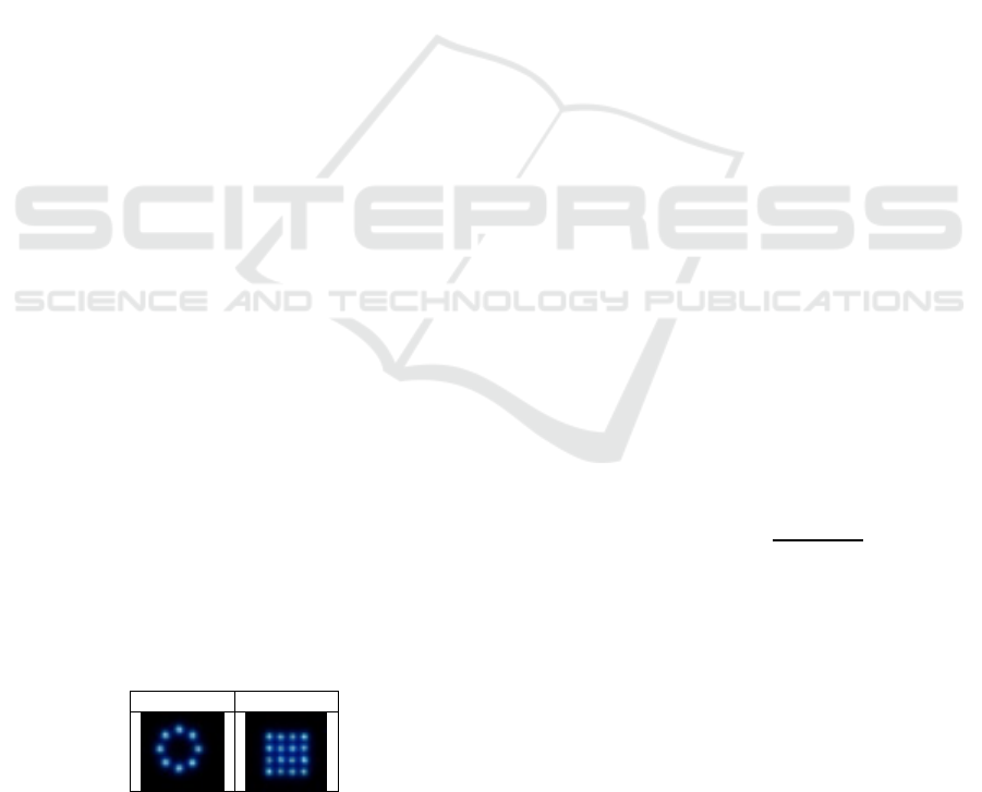
3.2 Constellation Images

Table 1: Sample of 3-Channel images.

8PSK 16QAM

In RF digital communications the information

carrying signals are modulated onto a carrier

waveform before transmission. The carrier is

modified by a triplet of attributes consisting of the

carrier’s amplitude, phase, and frequency. Modifying

these parameters in relation to the information

bearing signal allows for the superposition of the

information onto the carrier for RF communications.

To visualize these digitally modulated waveforms,

constellation images in the complex in-phase and

quadrature plane are often used. A technique defined

by (Peng, 2017) uses constellation images to map the

complex real and imaginary components to generate

RGB 3-Channel images. The images are used as

inputs to CNN classifiers. Two 3-Channel image

examples shown in Table 1, generated per (Conn,,

2019). The first image is 8 phase shift keying (8PSK)

and the second is 16 quadrature amplitude modulation

(16QAM). It is clear the images are discernible for

classification.

3.3 Clusters, Centroids and Euclidian

A cluster defines a set of objects in which each object

is closer to or more similar to an example object that

defines the cluster than to the example of any other

cluster. Clusters of objects are also often referred to

as classes. For data with continuous attributes, the

representative example of a cluster is often referred to

as a centroid, and it is often defined as the average of

all the points in the cluster. To assign a point to the

closest centroid, a proximity measure that quantifies

the concept of "closest" for the specific data under

consideration must be defined. The Euclidean (L2)

distance is often used for real data points in the

Euclidean space and is the most widely used distance

measurement because it is preserved under

orthogonal transformations such as the Fourier

transform (Tan, 2006) (Der, 2013). Given two 

dimensional vectors  and  , where 





,



,…



 and 







,



,…





, the Euclidian

L2 Distance between them is defined as:





,

























(1)

3.4 Dynamic Online Growing Neural

Gas (DYNG)

Approaches based on topological feature maps such

as self-organizing maps (SOM) (Kohonen, 1990),

neural gas (NG) (Hohonen, 1982), and growing

neural gas (GNG) (Fritzke, 1995) have been

successfully applied to online clustering problems.

Although successful, their architectures do not allow

for the labelling of different classes of data presented

to the networks. To address this DYNG (Beyer, 2013)

ICAART 2020 - 12th International Conference on Agents and Artiﬁcial Intelligence

988

extends GNG by allowing for online training and

class labelling of known data presented to a GNG

network. Figure 1 depicts a simplified diagram of a

DYNG network. DYNG exploits labelled data (C1,

C2, and C3) during training to adapt the network

structure to the requirements of the classification task.

Figure 1: Dynamic Online Growing Neural Gas (DYNG).

While the network is in online training mode it

can be presented with labelled and unlabelled data.

The labelled data are clustered into a set of neurons

marked with the same label. All unlabelled data

presented to the network are labelled as “?” and the

generated associated neurons are also labelled as “?”.

Then using a relabelling strategy, DYNG allows for

latent online labelling of unlabelled data when future

inputs with a new label falls within a predefined

distance from the unlabelled neurons.

A key limitation of DYNG is it does not allow for

the distinct labelling of different “unknown” classes

of stimuli as they are presented to the network.

DYNG does not explicitly detect when the unlabelled

data entries are from different classes or from

different population distributions, and then label them

as such. It is only at a later time when DYNG is

presented with a newly labelled stimulus that some

subset of the “unknown” neurons that fall within the

criteria of distance measures are relabelled to the new

label name. The research herein will attempt to

address this by providing a mechanism to

immediately detect and cluster anomalies as they

occur online.

4 METHODOLOGY

4.1 Overall Approach

CNNs have been demonstrated in countless

applications as highly accurate classifiers. However,

they are brittle in the sense that once trained they

cannot adapt to processing anomalous data and will

fail under such circumstances. To address this, a

twofold approach has been taken. First, we make use

of transfer learning and take advantage of the feature

extraction expertise that pre-trained CNNs have

gained from training on massive amounts of data.

This is done by freezing the weights and biases of all

but the last fully connected layer of the CNNs.

Secondly, we remove the last fully connected

classification layer of the CNNs and replace it with an

adaptive classification layer capable of maintaining

the original accuracy of the CNN. This adaptive layer

also provides for online anomaly detection,

adaptation, and clustering (or categorization) of the

anomalies into new unknown classes. Three such

adaptive classification algorithms are presented in the

remaining sections.

4.2 Training and Test Data

For this study, the GoogleNet, AlexNet, ResNet,

Inception, and MobileNet CNN architectures were

used to get a sampling of performance across various

architectures. Transfer learning was used by replacing

the last 1000-class output layer of the pre-trained

CNN with a 9-class softmax output layer with the

weights and biases trained on the waveform data sets.

The original weights and biases of all other layers

were frozen. For this work only known data sets are

trained on and presented to the classifiers for testing.

As of the writing of this paper, the results of

anomalous stimuli data are not presented; however,

preliminary results have shown favourable

performance accuracies. This study focuses on how

accurate the adaptive classifiers are in classifying the

known data they were trained upon. For each known

class type, there were 750 training samples, and for

validation there were 300 samples. The training data

set consisted of sample sets from nine different

waveforms. The nine classes were bipolar phase shift

keying (BPSK), quadrature amplitude shift keying

(4ASK), quadrature phase shift keying (QPSK),

orthogonal quadrature phase shift keying (OQPSK),

8PSK, 16QAM, 32QAM, 64QAM, and Noise. Using

the approach detailed in (Conn, 2019) and (Peng,

2017) for training, the modulated waveforms were

used to generate the 3-Channel constellation images

as shown in Table 1. The simulated waveforms had

varying levels of White-Gaussian noise with SNRs

ranging from -6 dB to 14 dB.

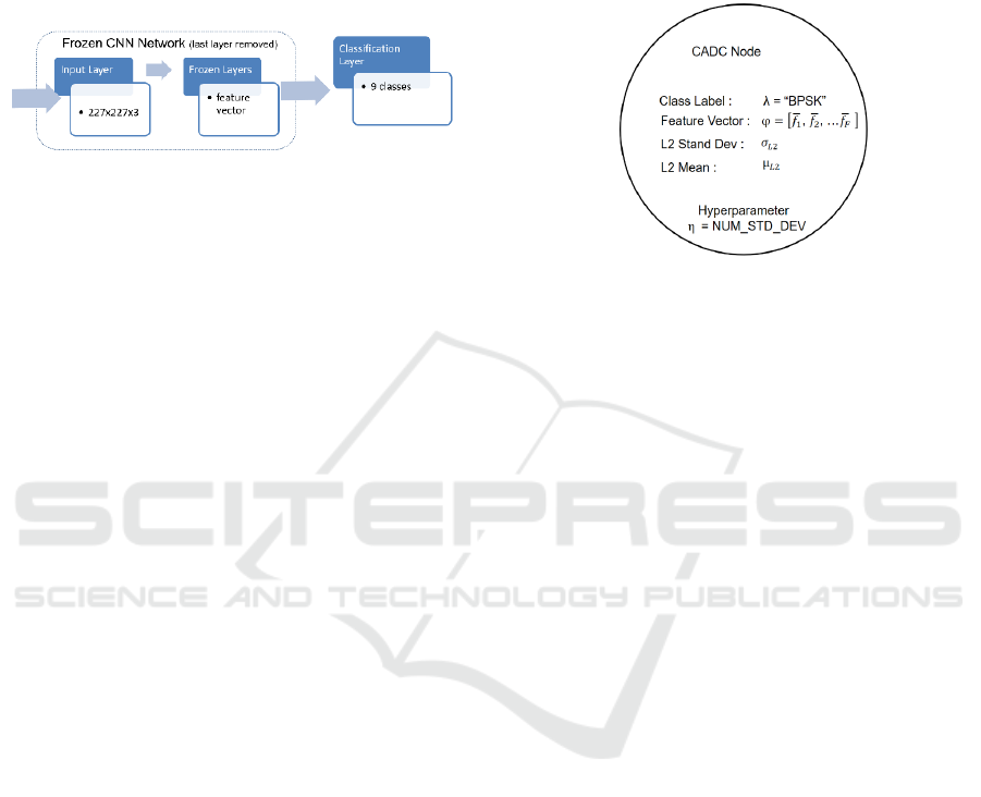
4.3 Baseline Accuracy Procedure

To establish the CNN-baseline accuracy, transfer

learning was used by replacing the last 1000-class

output layer of the pre-trained CNN with a 9-class

softmax output layer as shown in Figure 2. The

Adaptive Classiﬁers: Applied to Radio Waveforms

989

weights and biases of the new classification layer

were trained on the waveform data sets. Following the

training, accuracy of the networks was assessed using

the validation data. After the baseline accuracy of the

CNNs was established, the last 9-class layer of the

CNNs was removed and replaced with one of the

three adaptive classifiers discussed in section 4.4.

Figure 2: CNN Baseline Classifier.

Then each adaptive classifier was trained by

inputting the training data through the CNN

networks, therefore allowing the adaptive classifiers

to dynamically form their model structures. Then the

accuracy of the adaptive classifiers was determined

by using the validation data set.

4.4 Adaptive Classifiers

Three adaptive classifiers are explored in this

research: 1) Centroid with Anomaly Detection and

Clustering (CADC) algorithm; 2) Frequency Hits

Anomaly Detection and Clustering (FHITS-ADC);

and 3) DYNG Extended with CADC (DYNG-

CADC). For each of these algorithms the following

are defined: the specific model; the model training

phase; the online predictions, anomaly detection and

adaptation process; and finally the anomaly insertion

operation.

4.4.1 CADC Algorithm

The CADC algorithm is designed to perform class

predictions, anomaly detections, and semi-supervised

clustering (adaptation) functions. For each class, the

CADC algorithm generates a prototype node as

shown in Figure 3. The CADC prototypes have four

attributes. The class label λ defines the name of the

class (for example “BPSK”). φ defines a feature

vector of length N where each component defines the

mean of each corresponding feature from all training

data of the class. The φ dimension is of length N with

the value defined by the length of the CNN output

layer from which the centroid node takes input. φ is

considered the centroid of all training samples from

the same class. The L2 standard deviation 



and

mean 



establish boundaries on the use of the

centroid feature vector and play a significant role in

prediction decisions.

4.4.2 CADC Training

Before the CADC can perform classification,

anomaly detection, and anomaly clustering, it must

first be trained on C number of known training classes

to generate a CADC node for each known class.

Figure 3: CADC centroid node.

After training, the CADC will be composed of C

centroid nodes. Each centroid node will have a unique

label λ derived from the labelled training data and it

will have a feature vector φ. φ for each centroid is the

result of averaging the values at the corresponding

feature index positions from all training samples in

the same class. Once C prototype centroids are

established, the statistics 



and 



are computed.

This is done by reiterating through the training data

for each class and calculating the mean and standard

deviation of the L2 distances between a class centroid

and all training samples with the same class label.

Once trained, all centroids and associated statistics

for the known classes are defined, and the CADC

algorithm can then be taken online.

4.4.3 CADC Online Prediction &

Adaptation

With the trained CADC model taken online, it can

perform class predictions and adaptations when

anomalies are detected. As a stimulus is presented to

the centroid network, the L2 distance is computed

between the input stimulus and all centroid nodes.

The centroid with the smallest L2 distance is selected

as the candidate predicted class. To confirm

acceptance of the candidate, the number of standard

deviations hyper-parameter ( η is used. The L2

distance is checked to determine if the stimulus falls

within η standard deviations of the centroids (η=3

used for reported results). If the stimulus’ L2 distance

falls within the thresholds, it is accepted as classified.

If the stimulus is successfully declared as one of the

known classes, that prediction stands and no further

processing is required for that stimulus. However, if

ICAART 2020 - 12th International Conference on Agents and Artiﬁcial Intelligence

990

the stimulus is successfully predicted as one of the

unknown classes (as discussed in the next section),

the L2 standard deviation and mean statistic values

for that unknown class are updated. This action

provides for online refinement of the unknown class

statistics each time a stimulus is declared a particular

unknown class. If the incoming stimulus prediction is

rejected because the calculated L2 distance falls

outside of the selected centroid’s threshold, the

stimulus is declared and processed as an anomaly as

discussed in the next section.

4.4.4 CADC Anomaly Class Insertion &

Adaptation

The insertion of an unknown stimuli into the model is

a critical step of the adaptive learning process. When a

stimulus is declared an “anomaly” the goals are to: 1)

create a new unknown centroid class; 2) establish

prediction statistics for the new unknown class; and 3)

report the anomaly as a new unknown class. The

approach relies on the concept of one shot learning, and

the current statistics of all nodes of the CADC model.

When the first anomaly is detected a new centroid class

is created and labelled as “unknown1”, and when a

second anomaly is detected a new centroid class is

created and labelled as “unknown2”, etc. The feature

vector of the new unknown centroid is initialized to the

value of the stimulus vector. Then, to establish a model

on the new class, the statistical knowledge already

established on the centroids presently in the network

model is leveraged. In doing this, the L2 standard

deviation and mean for the new centroid is initialized

to be the average of all the L2 standard deviations and

means of all the existing centroid nodes. This average

includes averaging the statistics from the known and

unknown classes. Upon insertion completion, a new

unknown node has been generated with a reasonable

starting vector and statistics.

4.4.5 FHITS-ADC Algorithm

Figure 4: FHITS-ADC Node.

For each class, the FHITS-ADC algorithm generates

a prototype node as shown in Figure 4. The class label

λ defines the name of the class (for example

“BPSK”). The standard deviation (σ) and mean (μ)

vectors establish decision boundaries for predictions.

FHITS-ADC also requires two hyper-parameters, η

and β. The integer η defines the number of standard

deviations a feature vector’s components can fall

outside of boundary before an error is declared. The

real number β (can take on any value from 1.0 to 0) is

used to define the percentage of feature vector

components that can be in error before a stimulus is

declared an anomaly.

4.4.6 FHITS-ADC Training

The FHITS-ADC training algorithm begins with

generating labelled centroid nodes, 



. The nodes

have a class label, a standard deviation feature vector

(σ), and a mean feature vector (μ). The feature vector

dimension is defined by the length of the CNN output

layer that the centroid node will take input from (this

size is N). Before FHITS-ADC can be taken online, it

must first be trained on the C known classes.

Thereafter the FHITS-ADC model will consist of C

nodes. The μ feature vector is calculated similarly to

CADC. It is the result of averaging the values at the

corresponding feature index positions from all 



training samples within the same class. The σ feature

vector is the result of calculating the standard

deviation at the corresponding feature index positions

from all 



training samples within the same class.

4.4.7 FHITS-ADC Online Prediction and

Adaptation

With the trained network online, it can perform class

predictions, anomaly detection, and adaptation. As a





stimulus is presented to the network, the frequency

of error hits parameter  is computed

between the input stimulus and all class nodes in the

network. To carry out this computation, for all

centroid classes 



, each component of the stimulus

vector (









) is checked to determine if it falls within

η standard deviations of the component’s average

using the statistics computed during training. If a

corresponding value of the stimulus vector falls

outside the statistical limits,  is increased

indicating a non-match. The class with the least hits

is a candidate for the predicted class of the stimulus.

To confirm acceptance of the class prediction, the

hyper parameter threshold β is used. The β parameter

defines the maximum percentage of error hits allowed

before the stimulus is declared an anomaly. If the

stimulus’ hit counter falls below the threshold, the

Adaptive Classiﬁers: Applied to Radio Waveforms

991

stimulus is accepted as classified. If the stimulus is

successfully declared as one of the known classes

defined in the training set, then the prediction is

accepted. However, if the stimulus is predicted as an

unknown class (as discussed in the next section), the

mean statistic values are updated using the stimulus

value. This action provides for online refinement of

the unknown class statistics each time a stimulus is

declared as a particular unknown class. If the

incoming stimulus prediction is rejected because the

calculated hit counter falls above the threshold, the

stimulus is declared as an anomaly and insertion

processed as discussed in the next section.

4.4.8 FHITS-ADC Anomaly Insertion

When a stimulus is declared an “anomaly” the goals

are to: 1) create a new unknown node class; 2) quickly

establish prediction statistics for the new unknown

class; and 3) report the anomaly as a new unknown

class. To create unknown centroid classes, a running

index counter is used starting at value 1. When the

first anomaly is detected a new centroid class is

created and labelled as “unknown1”, and when a

second anomaly is detected a new centroid class is

created and labelled as “unknown2”, etc. To quickly

establish the centroid statistics, the feature vector of

the new unknown centroid is initialized to the value

of the stimulus vector. Then to establish a statistical

model of the new class, the knowledge already

established on the centroids presently in the network

model is leveraged by assigning the standard

deviation and mean vector of the new centroid to be

the average of all the standard deviations and means

of the statistics of all the existing centroid classes.

This includes averaging the statistics from the known

and unknown classes.

4.4.9 DYNG-CADC Algorithm

There is interest in exploring use of DYNG for online

streaming data classification because of its great

flexibility in adapting its structure to non-stationary

data while online. The strategy used is to extend (or

augment) the DYNG network with the CADC

algorithm to allow for the online rapid detection and

unique labelling of new anomaly classes as they are

input to the network. A similar approach could have

been taken by extending DYNG with FHITS-ADC.

The remainder of this subsection discusses DYNG

training and how CADC is used to extend the DYNG

network’s functionality.

4.4.10 DYNG-CADC Training

A complete description of the training algorithm for

DYNG is provided in (Beyer, 2013). Before the

DYNG-CADC algorithm is taken online, they both

must be trained on C known classes of training data.

The feature vector’s 



dimension is defined by the

length of the CNN’s output layer that the DYNG

nodes will take input from (this size is N).

After training, the initial DYNG model is

composed of C clusters of nodes representing the C

known classes. The number of nodes within each

cluster varies per class, and is determined

dynamically by the DYNG training algorithm. The

CADC network structure is also created and trained

on the training data set as described in the CADC

training section. In the DYNG-CADC algorithm, the

CADC structure is only used as an online adaptive

anomaly detector, and the DYNG network is used for

classification. It is expected (not proven) that the

DYNG network will provide greater classification

accuracy than CADC because it has multiple nodes

representing each class (therefore more voting power)

than CADC, which has only one node structure per

class. The hyper-parameters for the DYNG networks

are shown in Table 2. MAX_NODES was set to 100

nodes to limit the growth of the DYNG networks.

That yields approximately 11 DYNG nodes for each

of the 9 training classes. The MAX_AGE was set

relatively low to help minimize growth of the

network.

Table 2: DYNG Hyper-parameters.

EB0.1;EN0.0006;ALPHA0.5;D0.0005;

LAMBDA30;MAX_AGE25;

MAX_NODES100;NUM_STD5.0;

4.4.11 DYNG-CADC Online Prediction and

Adaptation

Once DYNG-CADC is trained on the known data set,

it can be taken online for classification, anomaly

detection, and clustering of unknown stimuli. In this

mode, CADC processes the stimuli first to determine

if the stimuli is declared an anomaly. If not declared

as such, DYNG is used to perform the stimuli

classification. If CADC declares the stimuli an

anomaly, a unique label is generated and the stimuli

with the new label is input to the DYNG in its training

mode to incorporate the new class into the network.

See section 4.4.1 for the CADC algorithm.

ICAART 2020 - 12th International Conference on Agents and Artiﬁcial Intelligence

992

5 EXPERIMENTAL RESULTS

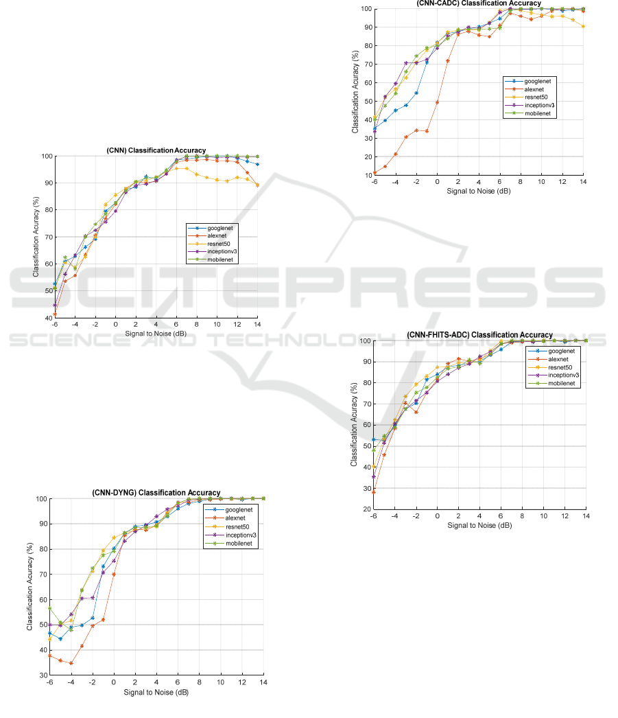
5.1 CNN Results

Figure 5 shows the performance of the five CNN

networks retrained for the nine classes. Overall, the

networks perform well. In general and as expected,

the accuracy of the classifiers increases as the SNR

increases. An unexpected observation for high SNRs

between 6 to 14 dB is that ResNet50, AlexNet, and

GoogleNet performances tend to drop, although their

overall performance is still above or near 90%. It is

not clear why these drops occur, as this behaviour

does not show itself in MobileNet and Inception. The

speculation is that additional training or hyper-

parameter adjustments on those networks will correct

for the degraded performance on the higher SNRs.

Figure 5: CNN Accuracy wrt. SNR.

5.2 CNN-DYNG Results

Figure 6 shows the overall classification performance

of the CNN-DYNG networks, with AlexNet

performing the least accurate and MobileNet

providing the best overall accuracy at about 85%.

Figure 6: CNN-DYNG Accuracy wrt. SNR.

5.3 CNN-CADC Results

CNN-DYNG generally performed better than the

CNN-CADC results, as shown in Figure 7 with

Inception for CNN-CADC giving the best

performance. For CNN-DYNG, MobileNet gives the

best performance. AlexNet consistently performed

the poorest.

Figure 7: CNN-CADC Accuracy wrt. SNR.

5.4 CNN-FHITS-ADC Results

The CNN-FHITS-ADC results in Figure 8 gives a

comparable performance to the other algorithms. It

stabilizes at about SNRs of 6 dB and above.

Figure 8 : CNN-FHITS-ADC Accuracy wrt. SNR.

5.5 Overall Accuracy Summary

Table 3 shows the overall performance of all algorithm

configurations. The top three performers are CNN-

FHITS-ADC-ResNet50, CNN-MobileNet, and CNN-

GoogleNet. In some cases, the standard softmax layer

for CNNs does not provide optimal classification

accuracy. For example, CNN-FHITS-ADC-ResNet50

provides greater performance (87.19%) than CNN-

Adaptive Classiﬁers: Applied to Radio Waveforms

993

resenet50 (83.63%). Another similar case is where

CNN-FHITS-ADC-AlexNet performance (84.63%) is

greater than CNN-AlexNet (84.10%).

Table 3: Overall Accuracy.

Orderby

Accuracy

Algorithm

Overall

Accuracy

1 CNN‐FHITS‐ADC‐ResNet50 87.19

2 CNN‐MobileNet 87.17

3 CNN‐GoogleNet 86.60

4 CNN‐FHITS‐ADC‐GoogleNet 86.24

5 CNN‐FHITS‐ADC‐MobileNet 86.24

6 CNN‐Inceptionv3 86.05

7 CNN‐DYNG‐MobileNet 85.33

8 CNN‐DYNG‐ResNet50 85.13

9 CNN‐FHITS‐ADC‐Inceptionv3 85.05

10 CNN‐CADC‐Inceptionv3 84.71

11 CNN‐FHITS‐ADC‐AlexNet 84.63

12 CNN‐CADC‐MobileNet 84.20

13 CNN‐AlexNet 84.10

14 CNN‐DYNG‐Inceptionv3 84.06

15 CNN‐CADC‐ResNet50 83.68

16 CNN‐ResNet‐50 83.63

17 CNN‐DYNG‐GoogleNet 82.68

18 CNN‐CADC‐GoogleNet 81.54

19 CNN‐DYNG‐AlexNet 79.11

20 CNN‐CADC‐AlexNet 70.67

However, use of these alternative last layer

classifiers does not guarantee greater performance

than softmax. For example, CNN-MobileNet using

the standard softmax layer outperforms all other

variants of MobileNet.

6 CONCLUSIONS

This work investigated using transfer learning and

adaptive classifiers for RF waveform classification

with various CNN architectures. This research

presented three online adaptive classifier frameworks

for the replacement of the last layer of CNNs to allow

for high accuracy classification performance in

nonstationary environments.

7 FUTURE WORK

Future research will investigate performance of the

online anomaly detection and adaptation capability of

these algorithms to demonstrate that such algorithms

can sustain acceptable accuracies in non-stationary

environments. Preliminary work has in fact shown that

these algorithms can provide acceptable performance.

ACKNOWLEDGEMENTS

We would like to thank Mr. Kwok Tom and Dr.

Anthony Martone of the Army Research Laboratory

for discussions on this topic.

REFERENCES

Conn, M., Darsana, D., 2019. Radio Frequency

Classification and Anomaly Detection using

Convolutional Neural Networks. IEEE Radar

Conference, Xplore.

Martone, A. F., et al., 2018. Spectrum Allocation for

Noncooperative Radar Coexistence. IEEE Transactions

on Aerospace and Electronic Systems.

Chaudhari, A., D. S., Tilghman, P., 2018. Colosseum: A

Battleground for AI Let Loose on the RF Spectrum.

Microwave Journal.

Peng, S., Jiang, H., Wang, H., Alwageed, H., Yao, D., 2017.

"Modulation classification using convolutional neural

network based deep learning model", 26th Wireless and

Optical Communication Conference.

Paul, B., Chiriyath, R., and Bliss, W., 2017. Survey of RF

Communications and Sensing Convergence Research.

IEEE Access.

Soekhoe, D., Plaat, A., 2016. On the Impact of Data Set Size

in Transfer Learning Using Deep Neural Networks.

Advances in Intelligent Data Analysis XV: 15th

International Symposium.

Beyer, O., 2013. Life-long Learning with Growing

Conceptual Maps. Phd Thesis. Technische Fakultat der

Universita Bielefeld.

Der, V., et al., 2013. "Change Detection in Streaming

Data". Ilmenau University of Technology, Dissertation.

Krizhevsky, A., I. Sulskever, and G.E. Hinton, 2012.

ImageNet Classification with Deep Convolutional

Neural Networks. Advances in Neural Information and

Processing Systems (NIPS).

Tang, Y.-J., Q.-Y. Zhang, and W. Lin, 2010. Artificial

Neural Network Based Spectrum Sensing Method for

Cognitive Radio. 6th International Conference on

Wireless Communications Networking and Mobile

Computing (WiCOM).

Ali, H., Zakieldeen, A., and Sulaiman, S., 2008. (Ldc S) for

Adaptation To Climate Change (Clacc) Climate

Change and Health in Sudan. (June).

Tan, N., Ning, Kumar, V, 2006. Introduction to Data

Mining. Pearson, Addison, Wesley

Fritzke, B., 1995. A Growing Neural Gas Network Learns

Topologies. Proceedings of International Conference

on Advances in Neural Information.

Kohonen, T., 1990. The Self-Organizing Map. Proceedings

of the IEEE Access.

Hohonen, T., 1982. Self-Organized Formation of

Topologically Correct Feature Maps. Springer-Verlag,

Biological Cybernetics.

ICAART 2020 - 12th International Conference on Agents and Artiﬁcial Intelligence

994