Reinforcement Learning in the Load Balancing Problem for the iFDAQ
of the COMPASS Experiment at CERN
Ond
ˇ
rej
ˇ
Subrt
1
, Martin Bodl
´
ak
2
, Matou
ˇ
s Jandek
1
, Vladim
´
ır Jar
´
y
1
, Anton
´
ın Kv
ˇ
eto
ˇ
n
2
, Josef Nov
´
y
1
,
Miroslav Virius
1
and Martin Zemko
1
1
Czech Technical University in Prague, Prague, Czech Republic
2
Charles University, Prague, Czech Republic
Keywords:
Data Acquisition System, Artificial Intelligence, Reinforcement Learning, Load Balancing, Optimization.
Abstract:
Currently, modern experiments in high energy physics impose great demands on the reliability, efficiency,
and data rate of Data Acquisition Systems (DAQ). The paper deals with the Load Balancing (LB) problem of
the intelligent, FPGA-based Data Acquisition System (iFDAQ) of the COMPASS experiment at CERN and
presents a methodology applied in finding optimal solution. Machine learning approaches, seen as a subfield
of artificial intelligence, have become crucial for many well-known optimization problems in recent years.
Therefore, algorithms based on machine learning are worth investigating with respect to the LB problem. Re-
inforcement learning (RL) represents a machine learning search technique using an agent interacting with an
environment so as to maximize certain notion of cumulative reward. In terms of RL, the LB problem is consid-
ered as a multi-stage decision making problem. Thus, the RL proposal consists of a learning algorithm using
an adaptive ε–greedy strategy and a policy retrieval algorithm building a comprehensive search framework.
Finally, the performance of the proposed RL approach is examined on two LB test cases and compared with
other LB solution methods.
1 INTRODUCTION
In 2014, the COMPASS (COmmon Muon Proton Ap-
paratus for Structure and Spectroscopy) (Alexakhin
et al., 2010) experiment at the Super Proton Syn-
chrotron (SPS) at CERN commissioned a novel, in-
telligent, FPGA-based Data Acquisition System (iF-
DAQ) (Bodlak et al., 2016; Bodlak et al., 2014) in
which event building is exclusively performed. Since
subevents are assembled in the FPGA cards (multi-
plexers (MUXes)) from ingoing data streams, these
data streams must be properly allocated to six MUXes
(up to eight in full setup) in order for the load to be
well-balanced in the system. Then complete events
are assembled from subevents in a specialized FPGA
card fulfilling the role of a switch. Finally, four
(up to eight in full setup) read out engine comput-
ers equipped with spillbuffer cards readout assembled
events and transfer them to CERN permanent storage
(CASTOR) (CERN, 2019).
This paper is organized as follows. Firstly, the
Load Balancing (LB) problem is given in Section 2.
Secondly, Section 3 gives a description of Rein-
forcement Learning (RL). In Subsection 3.1, the LB
problem is presented as a multi-stage decision mak-
ing problem. Subsection 3.2 defines the learning al-
gorithm and Subsection 3.3 shows the policy retrieval
algorithm. Both algorithms are combined in Subsec-
tion 3.4, finalizing the RL search framework.
Finally, the numerical results based on RL are
shown in Section 4 and are compared with other LB
solution methods.
2 LOAD BALANCING PROBLEM
For the iFDAQ, the most challenging task from the
LB point of view is load balancing at the multiplexer
(MUX) level. The optimization criterion is mini-
mization of the difference between the output flows
of the individual multiplexers. This minimization is
achieved by remapping the connection of inputs to
input ports of the multiplexers. Each input port es-
tablishes a connection between a data source (a de-
tector or a data concentrator) and the MUX level. For
the COMPASS experiment, it is necessary to consider
flows varying from 0 B to 10 kB for each input port.
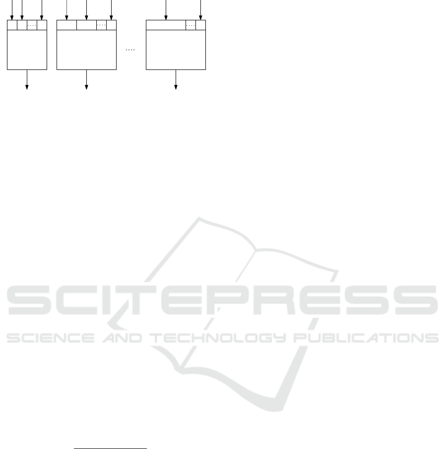
In Figure 1, a visualization of LB at the MUX
734
Šubrt, O., Bodlák, M., Jandek, M., Jarý, V., Kv
ˇ
eto
ˇ
n, A., Nový, J., Virius, M. and Zemko, M.
Reinforcement Learning in the Load Balancing Problem for the iFDAQ of the COMPASS Experiment at CERN.
DOI: 10.5220/0009035107340741
In Proceedings of the 12th International Conference on Agents and Artificial Intelligence (ICAART 2020) - Volume 2, pages 734-741
ISBN: 978-989-758-395-7; ISSN: 2184-433X
Copyright
c
 2022 by SCITEPRESS – Science and Technology Publications, Lda. All rights reserved

2
p
p + 1
p + 2
2p
1
MUX
1
MUX
2
MUX
m
(m − 1)p + 1
mp
f
k
1
f
k
2
f
k
p
f
k
p+1
f
k
p+2
f
k
2p
f
k
(m−1)p+1
f
k
mp
p
X
i=1
f
k
i
2p
X
i=p+1
f
k
i
mp
X
i=(m−1)p+1
f
k
i
Figure 1: Visualization of LB at the MUX level.
level is given. There are m MUXes with p ingoing
ports each. Moreover, n ∈ N flows f
k
1
, f
k
2
,..., f
k
mp
∈
N
0
, where n = m · p, are shown in the figure with in-
dices k
1
,k
2
,..., k
mp
∈ {i | 1 ≤ i ≤ n} ∧ ∀i, j : k
i
6= k
j
.
Despite the fact that each flow varies from 0 B
to 10 kB in the COMPASS experiment, the domain
N
0
is used. The motivation comes from a general ap-
proach to LB. Moreover, a flow with 0 B can be either
a physical connected input port sending no data or an
empty input port where no data source is connected
to. In brief, there are always n = m · p flows regard-
less whether all ports are used or not.
2.1 PROBLEM FORMULATION
Firstly, this subsection deals with a proper definition
of the LB problem.
Definition 1. Let m ∈ N denote the number of MUXes
with p ∈ N ingoing ports each, i.e., n = m · p ∈ N
ingoing ports in total and flows f
1
, f
2
,..., f
n
∈ N
0
.
Let S
1
,S
2
,..., S
m
be subsets of indices and F =
&
n
∑
i=1
f
i
/m
'
be a theoretical average flow for one
MUX. The Load Balancing (LB) problem is an op-
timization problem such that:
To minimize
v
u
u
t
m
∑
i=1
F −
∑
j∈S
i
f
j
!
2
, (1)
subject to the constraints
• each flow must be allocated
m
[
i=1
S
i
= {i | i ∈ 1,... ,n} (2)
• each flow must be allocated at most once
S
i
∩ S
j
=
/
0 ∀i, j = 1,..., m ∧ i 6= j (3)
• each MUX has p ports
|S
i
| = p ∀i = 1,..., m (4)
Secondly, a formulation of the index function is
given being helpful for the RL algorithms description.
Definition 2. Let S = {a
k
1
,a
k
2
,..., a
k
n
} be a set of
elements with indices k
1
,k
2
,..., k
n
∈ {i | 1 ≤ i ≤ n} ∧
∀i, j : k
i
6= k
j
. Function ϕ(i,S ) is the index function
such that
ϕ(i,S) = k
i
∀i = 1,... ,n. (5)
3 REINFORCEMENT LEARNING
Reinforcement Learning (RL) is a study of how ani-
mals and artificial systems can learn to optimize their
behaviour in the face of rewards and punishments
(Sutton and Barto, 1998; Szepesvari, 2010; Lapan,
2018). One way in which animals acquire complex
behaviours is by learning to obtain rewards and to
avoid punishments. During this learning process, the
agent interacts with the environment. At each step of
interaction, on observing or feeling the current state,
an action is taken by the learner (agent). Depending
on the goodness of the action at the particular situ-
ation, it is tried at the next stage when the same or
similar situation arises (Powell, 2007; Borrelli et al.,
2017; Busoniu et al., 2010). Finally, the best action at
each state or the best policy is manipulated based on
the observed rewards.
3.1 Load Balancing as a Multi-stage
Decision Making Problem
In order to view the LB problem as a multi-stage
decision making problem, the various stages of the
problem are to be identified. Consider a system with
n ∈ N flows f
1
, f
2
,..., f
n
∈ N
0
committed for allo-
cation to n = m · p ports. Then the LB problem in-
volves selecting p ∈ N flows to be allocated to the first
MUX from flows R
1
= { f
i
| i ∈ {1, ...,n}}, i.e., de-
termined by subset S
1
. For the second MUX, p flows
are selected from flows R
2
= { f
i
| i ∈ {1,... , n}}\S
1
}
and described by S
2
. The last, i.e., the m-th MUX
is occupied by remaining p flows R
m
= { f
i
| i ∈
{1,..., n}\
m−1
[
j=1
S
j
= S
m
} and in fact, there is no se-
lection procedure at all and the subset S
m
is deter-
mined directly. In general, the i-th MUX selects p
flows from flows R
i
= { f
j
| j ∈ {1,... , n}\
i−1
[
k=1
S
k
} and
a subset S
i
contains flow indices of the i-th MUX.
The problem statement follows. Initially, there are
p flows to be allocated in the i-th MUX chosen from
n − (i − 1)p flows. In this formulation, a flow to be
Reinforcement Learning in the Load Balancing Problem for the iFDAQ of the COMPASS Experiment at CERN
735

allocated at stage
k
is denoted as F
A
k
and is based on
an action a
k
. In RL terminology, the action a
k
corre-
sponds to a flow allocation either f
ϕ(k,R
i
)
or 0 to the
i-th MUX at stage
k
, i.e.,
F
A
k
=

0 if a
k
= 0
f
ϕ(k,R
i
)
if a
k
= 1.
(6)
Therefore, the action set A
k
consists of either 2
possibilities (allocate a
k
= 1 and do not allocate a
k
=
0) or 1 possibility (allocate a
k
= 1 or do not allocate
a
k
= 0) at stage
k
. That is,
A
k
= {a
min
k
,..., a
max
k
}, (7)
a
min
k
being the minimum possible action at stage
k
and
a
max
k
being the maximum possible action at stage
k
.
Values of a
min
k
and a
max
k
depend on the total flow
which has already been allocated at the previous k −1
stages, the number of flows already allocated, a flow
at the k-th stage and flows that can be allocated at the
remaining (n − (i − 1)p) − k stages.
The initial state is denoted as stage
1
. At stage
1
,
a decision is made on whether a flow f
ϕ(1,R
i
)
is allo-
cated or not. This action is denoted as a
1
and corre-
sponds to F
A
1
allocation at stage
1
.
Upon having made this decision, stage
2
is
reached. The expression (F
T
1
+ F
A
1
) represents the to-
tal flow which has already been allocated at the pre-
vious stages, i.e., stage
1
. At stage
2
, a decision a
2
is made on whether a flow f
ϕ(2,R
i
)
allocates or does
not allocate. Generally at stage
k
, a decision is made
on whether a flow f
k
is allocated or not. Finally,
stage
n−(i−1)p
is reached and a decision a
n−(i−1)p
is
made on whether a flow f
ϕ(n−(i−1)p,R
i
)
is allocated or
not.
Each state at any stage
k
can be defined as a tuple
(k, F
T
k
) where k is the stage number and F
T
k
is the total
flow which has already been allocated at the previous
k − 1 stages.
Thus for k = 1, the state information is denoted
as (1,F
T
1
) where F
T
1
is equal to 0 since no decision
concerning any flow allocation has been made so far.
The algorithm for the LB problem selects one among
the permissible set of actions and either allocates or
does not allocate a flow f
ϕ(1,R
i
)
at stage
1
so that it
reaches the next stage k = 2 with the total flow already
allocated and (n − (i − 1)p) − 1 flows for an alloca-
tion decision. Transition from (1,F
T
1
) on performing
an action a
1
∈ A
1
results in the next state reached as
(2,F
T
2
), where
F
T
2
= F
T
1
+ F
A
1
. (8)
Generally at stage
k
, from a state x
k
on performing
an action a
k
reaches a state x
k+1
, i.e., state transition
is from (k, F
T
k
) to (k + 1,F
T
k+1
), where
F
T
k+1
= F
T
k
+ F
A
k
. (9)
This repeats until the last stage. Therefore, a state
transition can be denoted as
x
k+1
= f (x
k
,a
k
), (10)
where f (x
k
,a
k
) is the function of state transition de-
fined by Equation 9.
Thus, the algorithm for the LB problem can be
treated as one of finding an optimum mapping from
the state space X to the action space A. The algorithm
design for the LB problem is finding or learning a
good or optimal policy (flows allocation) which is the
optimum allocation at each stage. Such allocation can
be treated as elements of an optimum policy π
∗
. For
finding the cost of allocation, it cumulates the costs at
each of the n − (i − 1)p stages of the problem. These
costs can be treated as a reward for performance of an
action in the perspective of the LB problem. The cost
of generation on following a policy π can be treated as
a measure of goodness of that policy. The Q–learning
technique is employed to cumulate costs and thus find
out the optimum policy.
For updating the Q value associated with the dif-
ferent state–action pairs, one should cumulate the to-
tal reward at different stages of allocation. In the
LB problem, the reward function g(x
k
,a
k
,x
k+1
) can
be chosen as −F
A
k
at stage
k
. The rewards are nega-
tive since Q–learning is considered as a minimization
problem. In the RL terminology, the immediate re-
ward is
r
k
= g(x
k
,a
k
,x
k+1
). (11)
Since the aim is to allocate as large as possible a
total flow, the estimated Q values of the state–action
pair are modified at each step of learning as
Q
s+1
(x
k
,a
k
) = Q
s
(x
k
,a
k
) + α[g(x
k
,a
k
,x
k+1
)
+ γ min
a
0
∈A
k+1
Q
s
(x
k+1
,a
0
) − Q
s
(x
k
,a
k
)].
(12)
Here, α is the learning parameter and γ is the dis-
count factor. When the system comes to the last stage
of decision making, there is no need of accounting
the future effects and then the estimate of Q value is
updated using the equation
Q
s+1
(x
k
,a
k
) = Q
s
(x
k
,a
k
) + α[g(x
k
,a
k
,x
k+1
)
− Q
s
(x
k
,a
k
)]. (13)
For finding an optimum policy, a learning algo-
rithm is designed. It iterates through each of the
n − (i − 1)p stages at each step of learning. As the
learning steps are carried out a sufficient number of
times, the estimated Q values of state–action pairs
will approach the optimum so that the optimum pol-
icy π
∗
(x) corresponding to any state x can be easily
retrieved.
ICAART 2020 - 12th International Conference on Agents and Artificial Intelligence
736

3.2 RL Algorithm for the LB Problem
using ε–greedy Strategy
In the previous subsection, the LB problem is formu-
lated as a multi-stage decision making problem. To
find the best policy or the best action corresponding
to each state, the RL technique is used. The solution
consists of two phases, namely the learning phase and
the policy retrieval phase.
To carry out the learning task, one issue concerns
how to select an action from the action space. In this
subsection, the ε–greedy strategy of exploring action
space is used.
Instead of choosing all actions several times, it
makes sense to choose the actions which may be the
best action. The greedy action is chosen with a proba-
bility (1−ε) and one of the other actions with a prob-
ability ε. The greedy action a
g
k
corresponds to the ac-
tion with the best estimate of the Q value at stage
k
,
i.e.,
a
g
k
= argmin
a∈A
k
Q
s
(a). (14)
It may be noted that if ε = 1, the algorithm will
select one of the actions with uniform probability and
if ε = 0, the greedy action will be selected. Initially,
the estimates Q
s
(a) may be far from their true value.
However as s → ∞, Q
s
(a) → Q(a), the information
contained in Q
s
(a) becomes increasingly exploitable.
So in the ε–greedy algorithm, initially ε is chosen
close to 1 and as s increases, ε is gradually reduced.
Finally, proper balancing of exploration and exploita-
tion of the action space ultimately reduces the number
of trials needed to find the best action.
For solving this multi-stage problem using RL, the
first step is fixing of state space X and action space
A precisely. The whole concept for the i-th MUX is
explained in a general way, where the number of flows
is n − (i − 1)p.
The fixing of state space X primarily depends on
the number of flows and the possible values of the
total flow in the i-th MUX (which in turn directly de-
pends on the minimum and maximum values of each
flow). Since there are n − (i − 1)p stages for solution
of the problem, the state space is also divided into
n − (i − 1)p subspaces. Thus, if there are n − (i − 1)p
flows to be allocated, then
X = X
1
∪ X
2
∪ . .. ∪ X
n−(i−1)p
. (15)
The allocation problem should go through n−(i−
1)p stages for making decision to allocate or not to
allocate for each of the n − (i − 1)p flows. At any
stage
k
, the part of state space to be considered X
k
con-
sists of the different tuples having the stage number
as k and the total flow already allocated varying from
F
Tmin
k
to F
Tmax
k
, where F
Tmin
k
is the minimum possible
total flow already allocated and F
Tmax
k
the maximum
possible total flow already allocated at the previous
k − 1 stages. Thus,
X
k
= {(k,F
Tmin
k
),..., (k,F
Tmax
k
)}, (16)
where F
Tmin
k
is the minimum possible total flow
already allocated at the previous k − 1 stages, i.e.,
F
Tmin
k
= 0 (17)
and F
Tmax
k
is the maximum possible total flow al-
ready allocated at the previous k − 1 stages, i.e.,
F
Tmax
k
=
k−1
∑
j=1
f
ϕ( j,R
i
)
. (18)
At each step, the LB problem algorithm will se-
lect an action from the permissible set of actions and
forward the system to one among the next permissi-
ble states. Therefore, the action set A
k
is a dynami-
cally varying one, depending on the flows already al-
located at the previously considered stages. As the
number of MUXes or number of ports in each MUX
increases, the number of states in the state space in-
creases. Thus, state space and action space are both
discrete.
The action set A
k
consists of either 2 possibil-
ities (allocate a
k
= 1 and do not allocate a
k
= 0)
or 1 possibility (allocate a
k
= 1 or do not allocate
a
k
= 0) at stage
k
. At the current state x
k
, the ac-
tion set A
k
depends on the total flow already allocated
F
T
k
, the number of flows already allocated p
A
, a flow
at the k-th stage f
ϕ(k,R
i
)
and flows that can be allo-
cated at the remaining (n − (i − 1)p) − k stages, i.e.,
f
ϕ(k+1,R
i
)
,..., f
ϕ(n−(i−1)p,R
i
)
. Therefore, the action set
A
k
is dynamic in nature in the sense that it depends
on the total flow already allocated up to that stage and
also the number of flows already allocated at the pre-
vious k − 1 stages. If F
T
k
is the total flow already al-
located, p
A
is the number of flows already allocated,
f
ϕ(k,R
i
)
is a flow at stage
k
, the minimum value and the
maximum value of action a
k
are defined as
a
min
k
=























0 if p = p
A
0 if F −F
T
k
< f
ϕ(k,R
i
)
0 if p − p
A
< (n − (i − 1)p) − k ∧
F −F
T
k
< L
p−p
A
−1,(n−(i−1)p)−k
+ f
ϕ(k,R
i
)
0 if p − p
A
< (n − (i − 1)p) − k ∧
F −F
T
k
≥ L
p−p
A
,(n−(i−1)p)−k
1 otherwise,
a
max
k
=















0 if p = p
A
0 if F −F
T
k
< f
ϕ(k,R
i
)
0 if p − p
A
< (n − (i − 1)p) − k ∧
F −F
T
k
< L
p−p
A
−1,(n−(i−1)p)−k
+ f
ϕ(k,R
i
)
1 otherwise,
(19)
Reinforcement Learning in the Load Balancing Problem for the iFDAQ of the COMPASS Experiment at CERN
737

where L
u,v
denotes the sum of the u smallest flows
at last v stages. Below, Equation 19 is discussed in
more detail.
The conditions F − F
T
k
< f
ϕ(k,R
i
)
and p = p
A
are
common for both a
min
k
and a
max
k
. Clearly, if a flow
f
ϕ(k,R
i
)
at stage
k
is greater than F − F
T
k
(the rest what
remains to allocate), it does not allow the flow f
ϕ(k,R
i
)
to be allocated at stage
k
. Similarly, if the number of
flows already allocated p
A
is equal to the number of
ports p, there is no free port available for a flow allo-
cation. Therefore, both a
min
k
and a
max
k
are equal to 0 if
the condition is true.
The second condition p− p
A
< (n−(i−1)p)−k∧
F − F
T
k
< L
p−p
A
−1,(n−(i−1)p)−k
+ f
ϕ(k,R
i
)
is also com-
mon for both a
min
k
and a
max
k
. The condition examines
whether the flow f
ϕ(k,R
i
)
has to be necessarily allo-
cated or not. The first part, p − p
A
< (n − (i − 1)p) −
k, checks whether there are enough flows at the re-
maining (n −(i−1)p)−k stages to fill remaining free
ports if the flow f
ϕ(k,R
i
)
is not to be allocated. The
second part, F −F
T
k
< L
p−p
A
−1,(n−(i−1)p)−k
+ f
ϕ(k,R
i
)
,
checks if the flow f
ϕ(k,R
i
)
together with the sum of the
p − p
A
−1 smallest flows at the last (n−(i−1)p)−k
stages are higher than F − F
T
k
, ensuring that the total
i-th MUX flow is less or equal than F. If both parts
are satisfied, both a
min
k
and a
max
k
are equal to 0.
The last condition deals with a
min
k
only. The
condition p − p
A
< (n − (i − 1)p) − k ∧ F − F
T
k
≥
L
p−p
A
,(n−(i−1)p)−k
consists of two parts. The first part,
p − p
A
< (n − (i − 1)p) − k, checks again whether
there are enough flows at the remaining (n − (i −
1)p) − k stages to fill remaining free ports if the
flow f
ϕ(k,R
i
)
is not to be allocated. The second part,
F −F
T
k
≥ L
p−p
A
,(n−(i−1)p)−k
, determines whether the
sum of the p − p
A
smallest flows at the last (n −
(i − 1)p) − k stages is less than F − F
T
k
, ensuring
that the total i-th MUX flow is less or equal than F.
If both parts are satisfied, the flow f
ϕ(k,R
i
)
does not
necessarily have to be allocated, since all LB prob-
lem conditions can be still satisfied at the remaining
(n − (i − 1)p) − k stages.
Clearly, if none of the above-mentioned condi-
tions is satisfied, both a
min
k
and a
max
k
are equal to 1 and
the flow f
ϕ(k,R
i
)
has to be allocated in the i-th MUX.
To conclude, if F − F
T
k
< f
ϕ(k,R
i
)
or p = p
A
is
satisfied, the choice can only be made from one ac-
tion – do not allocate a
k
= 0. There is also no
choice if p − p
A
< (n − (i − 1)p) − k ∧ F − F
T
k
<
L
p−p
A
−1,(n−(i−1)p)−k
+ f
ϕ(k,R
i
)
is true, since it leads
to only one possible action again – do not allocate
a
k
= 0.
The situation when two actions are feasible (allo-
cate a
k
= 1 and do not allocate a
k
= 0) depends on
the condition p − p
A
< (n − (i − 1)p) − k ∧ F − F
T
k
≥
L
p−p
A
,(n−(i−1)p)−k
. The decision to allocate the flow
f
ϕ(k,R
i
)
can be seen as a substitution of the (p − p
A
)-th
smallest flow at last (n − (i − 1)p) − k stages for the
flow f
ϕ(k,R
i
)
.
All other situations lead to both a
min
k
and a
max
k
be-
ing equal to 1 and the only one possible decision is to
allocate the flow f
ϕ(k,R
i
)
in the i-th MUX.
Algorithm 1: Learning algorithm for the LB problem of the
i-th MUX using ε–greedy strategy.
1: load flows R
i
, average flow F
2: set the learning parameter α, the discount factor γ
and the greedy factor ε
3: set the maximum iteration s
max
4: set Q values to zeros
5: for i = 1 → n − (i − 1)p do  stages initialization
6: X
i
= initStage(i)
7: for all x
k
∈ X
i
do  states initialization
8: a
min
k
= getMinAction()  see Eq. 19
9: a
max
k
= getMaxAction()  see Eq. 19
10: setStatePermissibleActions(x
k
,a
min
k
,a
max
k
)
11: end for
12: end for
13: for s = 1 → s
max
do  learning phase
14: F
T
1
= 0, p
A
= 0
15: for k = 1 → n − (i − 1)p do
16: x
k
= getCurrentState(k, F
T
k
)
17: A
k
= getActions(k, x
k
,F, p
A
)  see Eq. 19
18: a
k
= getGreedyAction(Q,A
k
,ε)
19: p
A
= p
A
+ a
k
20: F
T
k+1
= F
T
k
+ f
ϕ(k,R
i
)
· a
k
21: if k < n − (i − 1)p then
22: Q = updateQ(Q, x
k
,a
k
)  see Eq. 12
23: else
24: Q = updateQ(Q, x
k
,a
k
)  see Eq. 13
25: end if
26: end for
27: set the greedy factor ε = 1 − s/s
max
28: end for
The learning procedure can now be summarized,
see Algorithm 1. Initially, the total flow already al-
located is set to 0 at stage
1
. Then an action is per-
formed that either allocates or not the flow at stage
1
and then it proceeds to the next stage (k = 2) with the
total flow already allocated. This proceeds until all
the n − (i − 1)p flows are either allocated or not. At
each state transition step, the estimated Q value of the
state–action pair is updated using Equation 12.
As the learning process reaches the last stage,
a flow at stage
n−(i−1)p
is either allocated or not. Then
ICAART 2020 - 12th International Conference on Agents and Artificial Intelligence
738

the Q value is updated using Equation 13. The tran-
sition process is repeated a sufficient number of times
(iterations) and each time the allocation process goes
through all the n − (i − 1)p stages.
Algorithm 2: Policy retrieval algorithm for the LB problem
of the i-th MUX using RL.
1: load flows R
i
, average flow F, Q values
2: F
T
1
= 0, p
A
= 0
3: S
i
= {}
4: for k = 1 → n − (i − 1)p do  retrieval phase
5: x
k
= getCurrentState(k, F
T
k
)
6: A
k
= getActions(k, x
k
,F, p
A
)  see Eq. 19
7: a
g
k
= argmin
a∈A
k
Q(x
k
,a)
8: if a
g
k
= 1 then
9: S
i
= S
i
∪ ϕ(k,R
i
)
10: end if
11: p
A
= p
A
+ a
g
k
12: F
T
k+1
= F
T
k
+ f
ϕ(k,R
i
)
· a
g
k
13: end for
3.3 Policy Retrieval
After the learning phase is done, the retrieval phase
begins. The system is learnt and the learnt values are
stored in a lookup table. The retrieval phase accesses
the lookup table in order to retrieve the required re-
sults. The learnt values in the lookup table can be
used unless the parameters of the system change. In
this case, the system must be learnt again by trigger-
ing a new run of learning phase.
As the learning proceeds, and the Q values of
state-action pairs are updated, Q
s
approaches Q
∗
.
Next, the optimum Q
s
values are used to obtain the
optimum allocation. The retrieval algorithm is sum-
marized in Algorithm 2. At stage
1
, F
T
1
= 0 is ini-
tialized and thus, the state of the system is (1,F
T
1
).
The algorithm finds the greedy action at this stage as
a
g
1
which is the best allocation F
A
1
for stage
1
. The
retrieval algorithm reaches the next state as (2,F
T
2
)
where F
T
2
= F
T
1
+ a
g
1
· f
ϕ(1,R
i
)
and finds the greedy
action corresponding to stage
2
as a
g
2
. This proceeds
up to stage
n−(i−1)p
. Finally, a set of actions (allo-
cations) a
g
1
,a
g
2
,..., a
g
n−(i−1)p
is obtained, which is the
optimum allocation F
A
1
,F
A
2
,..., F
A
n−(i−1)p
for the i-th
MUX. Thus, it builds up the subset S
i
= {ϕ( j, R
i
) |
F
A
j
6= 0 ∀ j = 1,..., n − (i − 1)p}.
3.4 Complete Algorithm
Finally, an algorithm considering all m ∈ N MUXes
is proposed, see Algorithm 3. The idea is to learn
and retrieve S
1
for the first MUX, then reduce a set of
flows R
1
by the allocated flows and get a set of flows
R
2
for the second MUX, etc. Generally, the i-th MUX
is learnt, S
i
is retrieved and R
i
is reduced by S
i
giving
R
i+1
for the (i+1)-th MUX. Regarding the last MUX,
the m-th MUX, a set R
m
determines directly S
m
.
Algorithm 3: The complete LB problem algorithm consid-
ering m MUXes using RL.
1: load flows R
1
2: for i = 1 → m − 1 do  get LB of the i-th MUX
3: F =
&
n−(i−1)p
∑
j=1
f
ϕ( j,R
i
)
/(m − i + 1)
'
4: Q = learningPhase(R
i
,F)  see Alg. 1
5: S
i
= retrievalPhase(R
i
,F, Q)  see Alg. 2
6: R
i+1
= { f
j
| j ∈ {1,... ,n}\
i
[
k=1
S
k
}
7: end for
8: S
m
= {ϕ( j, R
m
) | ∀ j = 1, ..., p}
4 NUMERICAL RESULTS
The RL approach has been implemented in C++
and Matlab (R2018a, 64-bit) on a personal computer
equipped with Intel(R) Core(TM) i7-8750H CPU
(@2.20 GHz, 6 Cores, 12 Threads, 9M Cache, Turbo
Boost up to 4.10 GHz) and 16 GB RAM (DDR4,
2 666 MHz) memory. The RL approach is examined
on two test cases and numerical results are compared
with other methods of solving the LB problem.
The results are investigated with respect to the er-
ror and computation time. The error is defined as the
objective function of the LB problem, see Equation 1.
4.1 Test Case 1
The Test Case 1 (TC1) consists of m = 6 MUXes with
p = 15 ingoing ports each. It corresponds to the iF-
DAQ setup used in the Run 2016, 2017 and 2018. It
considers n = m · p = 6 · 15 = 90 flows with values
randomly generated in the range from 0 B to 10 kB.
The proposed RL algorithm is strongly stochastic
and hence, it produces a unique solution in every ex-
ecution. The parameters used for the RL algorithm to
solve the TC1 are given in Table 1. The quality of the
results depends on s
max
directly controlling how well
state–action pairs are learnt represented by Q values.
The s
max
setup requires experience of an executor.
In Table 2, the results produced in C++ and Mat-
lab for the TC1 using RL in each execution are stated.
Reinforcement Learning in the Load Balancing Problem for the iFDAQ of the COMPASS Experiment at CERN
739

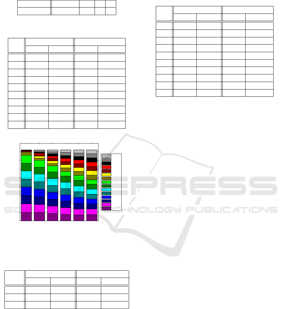
Table 1: Parameters used for the RL algorithm.
Parameter s
max
α γ ε
Value 100,000 0.1 1 1
Table 2: The TC1 results using the RL approach in each
execution.
Ex.
C++ Matlab
Error t [ms] Error t [ms]
1 10.44 32,404 10.44 117,253
2 10.44 32,515 10.44 117,252
3 10.44 32,761 10.44 117,106
4 10.44 32,961 10.44 119,307
5 10.44 33,357 10.44 119,113
6 10.44 34,818 10.44 117,690
7 10.44 35,409 10.44 118,236
8 10.44 34,544 10.44 118,427
9 10.44 35,130 10.44 118,242
10 10.44 36,324 10.82 117,918
82,494
82,492
82,486
82,491
82,498 82,498
MUX
1
MUX
2
MUX
3
MUX
4
MUX
5
MUX
6
0
10,000
20,000
30,000
40,000
50,000
60,000
70,000
80,000
90,000
Flow [B]
Port 15
Port 14
Port 13
Port 12
Port 11
Port 10
Port 9
Port 8
Port 7
Port 6
Port 5
Port 4
Port 3
Port 2
Port 1
Figure 2: The same best TC1 flow allocation based on RL
produced in C++ (Execution 1) and Matlab (Execution 3).
Table 3: Comparison of LB solution methods based on the
best flow allocation for the TC1.
Met.
C++ Matlab
Error t [ms] Error t [ms]
GH 243.89 47 243.89 1
ILP 21.19 17,127 23.81 1,465
RL 10.44 32,404 10.44 117,106
The error is equal approximately to 10.44 giving a so-
lution close to the global optimum in each execution.
In Figure 2, the same best TC1 flow allocation pro-
duced in C++ (Execution 1) and Matlab (Execution
3) is shown. Moreover, a comparison of the lowest
total flow allocation and highest total flow allocation
for the respective MUXes might be performed. The
third MUX has the lowest total flow allocation with
value of 82,486 B and on the other hand, the fifth and
Table 4: The TC2 results using the RL approach in each
execution.
Ex.
C++ Matlab
Error t [ms] Error t [ms]
1 11.23 59,566 11.66 206,358
2 7.07 61,716 5.29 203,017
3 11.66 63,979 6.48 203,287
4 11.31 66,219 11.22 204,427
5 11.31 74,745 6.32 207,476
6 6.48 77,605 11.22 208,410
7 7.87 79,134 2.45 204,824
8 11.66 80,781 6.16 205,160
9 2.83 75,882 11.49 204,299
10 11.23 76,138 11.14 204,525
sixth MUX have the highest total flow allocation with
a value of 82,498 B each. The ratio of the flows is
82,486/82,498 ≈ 99.99%.
In order to calculate an optimal solution, Matlab
consumes several times more computational time than
a version implemented in C++. The high computa-
tional time for Matlab comes from a type of opera-
tion required in an optimization process. In RL, the
main mathematical operations are performed on sub-
matices of matrices, e.g., sum of elements, minimum
or maximum from elements of a submatrix. In C++,
pointers are a very efficient way how to implement
such mathematical operations. Since pointers are ab-
sent in Matlab, a submatrix must be always copied to
perform a particular mathematical operation.
However, the computational time for both C++
and Matlab is quite high, resulting in an exclusion of
the RL algorithm as a real-time LB solver. On the
other hand, the error is quite small. Therefore, the RL
approach can be considered for a long-term LB setup,
where no frequent changes in the flows are expected.
The proposed RL algorithm is compared with
other LB solution methods – Greedy Heuristic (GH)
and Integer Linear Programming (ILP) – in Table 3.
4.2 Test Case 2
The Test Case 2 (TC2) consists of m = 8 MUXes with
p = 15 ingoing ports each and thus, it corresponds
to the iFDAQ full setup. However, the iFDAQ full
setup has never been in operation for the COMPASS
experiment since it was not required by any physics
program. It considers n = m · p = 8 · 15 = 120 flows
with values randomly generated in the range from 0 B
to 10 kB. The parameters used for the RL algorithm
to solve the TC2 are the same as for TC1, see Table 1.
In Table 4, the results produced in C++ and Mat-
lab for the TC2 using RL in each execution are stated.
ICAART 2020 - 12th International Conference on Agents and Artificial Intelligence
740

68,401
68,399
68,401 68,401 68,401
68,399
68,401 68,401
MUX
1
MUX
2
MUX
3
MUX
4
MUX
5
MUX
6
MUX
7
MUX
8
0
10,000
20,000
30,000
40,000
50,000
60,000
70,000
Flow [B]
Port 15
Port 14
Port 13
Port 12
Port 11
Port 10
Port 9
Port 8
Port 7
Port 6
Port 5
Port 4
Port 3
Port 2
Port 1
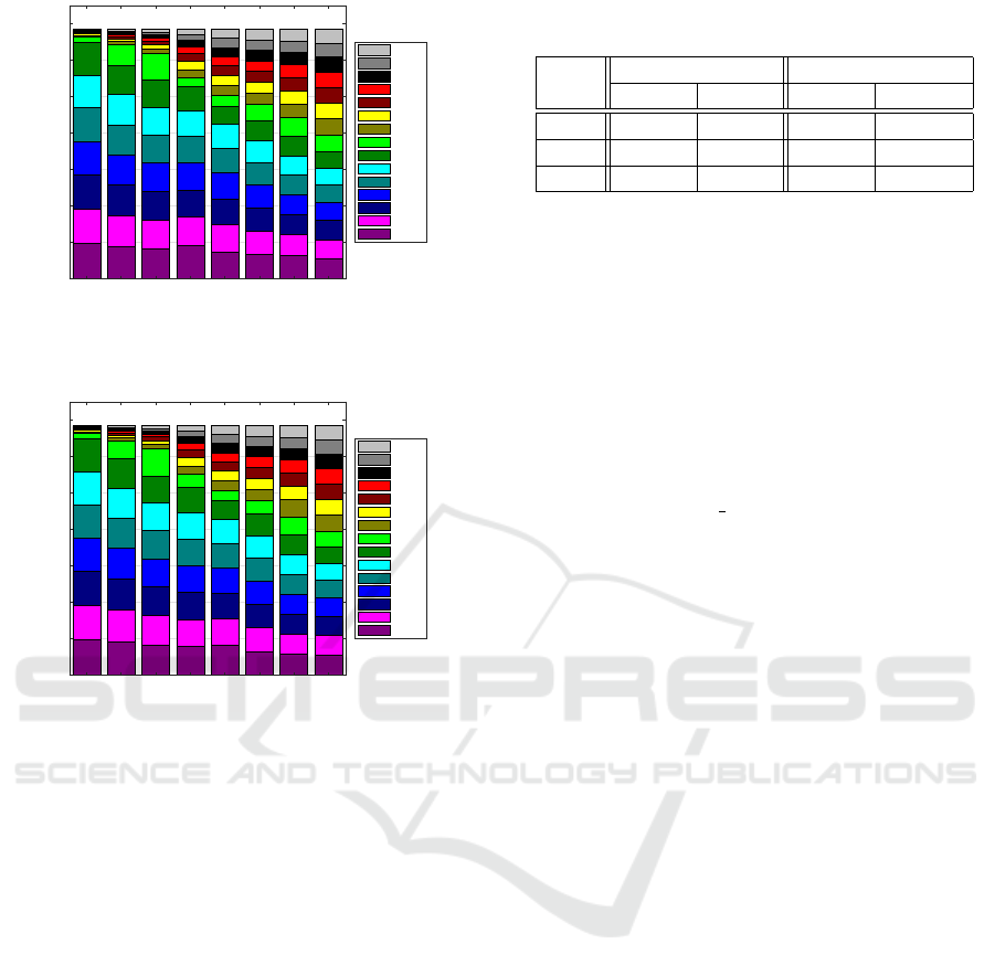
Figure 3: The best TC2 flow allocation based on RL pro-
duced in C++ corresponding to Execution 9.
68,401
68,400
68,401
68,399
68,401 68,401 68,401
68,400
MUX
1
MUX
2
MUX
3
MUX
4
MUX
5
MUX
6
MUX
7
MUX
8
0
10,000
20,000
30,000
40,000
50,000
60,000
70,000
Flow [B]
Port 15
Port 14
Port 13
Port 12
Port 11
Port 10
Port 9
Port 8
Port 7
Port 6
Port 5
Port 4
Port 3
Port 2
Port 1
Figure 4: The best TC2 flow allocation based on RL pro-
duced in Matlab corresponding to Execution 7.
The best TC2 flow allocation based on RL produced
in C++ corresponding to Execution 9 is given in Fig-
ure 3 and produced in Matlab corresponding to Exe-
cution 7 is given in Figure 4. In almost each execu-
tion, a unique solution is retrieved giving very precise
LB with the small error. Finally, the TC2 results pro-
duced by RL are compared with results acquired by
GH and ILP in Table 5.
5 CONCLUSION
The paper has introduced the LB problem of the iF-
DAQ of the COMPASS experiment at CERN. RL
refers to a kind of machine learning method in which
an agent receives a delayed reward in the next time
step to evaluate its previous action.
The high computational time and the low error
cause the proposed RL approach to be more fitting for
a long-term LB setup, where no frequent changes in
the flows are expected. In addition, the RL approach
might lead to a quite high RAM memory consumption
Table 5: Comparison of LB solution methods based on the
best flow allocation for the TC2.
Met.
C++ Matlab
Error t [ms] Error t [ms]
GH 224.22 63 224.22 1
ILP 194.43 49,927 134.61 95,251
RL 2.83 75,882 2.45 204,824
during execution to store values of each state, since
the problems can be quite complex.
Thus, a question of real-time LB is still open and
requires further investigation.
ACKNOWLEDGEMENTS
This research has been supported by OP
VVV, Research Center for Informatics,
CZ.02.1.01/0.0/0.0/16 019/0000765.
REFERENCES
Alexakhin, V. Y. et al. (2010). COMPASS-II Proposal. The
COMPASS Collaboration. CERN-SPSC-2010-014,
SPSC-P-340.
Bodlak, M. et al. (2014). FPGA based data acquisition sys-
tem for COMPASS experiment. Journal of Physics:
Conference Series, 513(1):012029.
Bodlak, M. et al. (2016). Development of new data ac-
quisition system for COMPASS experiment. Nuclear
and Particle Physics Proceedings, 273(Supplement
C):976–981. 37th International Conference on High
Energy Physics (ICHEP).
Borrelli, F., Bemporad, A., and Morari, M. (2017). Pre-
dictive Control for Linear and Hybrid Systems. Cam-
bridge University Press, Cambridge, UK, first edition.
Busoniu, L., Babuska, R., Schutter, B. D., and Ernst,
D. (2010). Reinforcement Learning and Dynamic
Programming Using Function Approximators. CRC
Press, Boca Raton, Florida.
CERN (2019). CASTOR — CERN Advanced Storage man-
ager.
Lapan, M. (2018). Deep Reinforcement Learning Hands-
On: Apply modern RL methods, with deep Q-
networks, value iteration, policy gradients, TRPO, Al-
phaGo Zero and more. Packt Publishing, Birming-
ham, UK. ISBN 1788834240.
Powell, W. B. (2007). Approximate Dynamic Programming.
Willey-Interscience, New York. ISBN 0470171553.
Sutton, R. S. and Barto, A. G. (1998). Reinforcement Learn-
ing: An Introduction. MIT Press, Cambridge, MA.
ISBN 0262193981.
Szepesvari, C. (2010). Algorithms for Reinforcement Learn-
ing. Morgan and Claypool Publishers, San Rafael,
California. ISBN 1608454924.
Reinforcement Learning in the Load Balancing Problem for the iFDAQ of the COMPASS Experiment at CERN
741