
Adaptive Modelling of Fed-batch Processes with Extreme Learning
Machine and Recursive Least Square Technique
Kazeem Alli and Jie Zhang
School of Engineering, Merz Court, Newcastle University,
Newcastle upon Tyne NE1 7RU, U.K.
Keywords: Extreme Learning Machine, Neural Networks, Fed-batch Processes, Recursive Least Square, Model
Parameter Estimation, Optimization Control.
Abstract: This paper presents a new strategy to integrate extreme learning machine (ELM) with recursive least square
(RLS) technique for the adaptive modelling of fed-batch processes that are subject to unknown disturbances.
ELM has the advantage of fast training and good generalization. ELM is effective in modelling nonlinear
processes but faces problems when the modelled process is time varying due to the presence of unknown
disturbances or process condition drift. The RLS can adapt to current process operation by recursively solving
the least square problem in the considered model. The RLS estimation algorithm nullifies the model plant
mismatches caused by the unknown disturbances through correction of parameter estimates at each iteration.
The offline trained output layer weights of an ELM are used as the initial values in parameter estimation in
RLS, which are being updated after each batch run using RLS. The proposed strategy is tested on an
isothermal semi-batch reactor. The results obtained show that the proposed batch to batch adaptive modelling
technique is very effective.
1 INTRODUCTION
Fed-batch processes are a commonly used production
technique for the manufacturing of high value-added
products such as specialty chemicals and
pharmaceuticals (Bonvin, 1998; Ruppen et al., 1995).
Both fed batch and batch processes operate in similar
pattern only that the intermittent addition of the
reactants is not required in the case of batch
operation.
These process operations possess great benefit in
many manufacturing industries as they help to
ascertain controlled situation during the progress of a
reaction whereby operating variables, such as the
feed-rate, temperature, pressure, and agitation rate are
varied according to a specified dynamic or steady
trajectory. According to (Xiong and Zhang, 2005),
the significant requirement of batch process
optimization is the accurate mathematical
representation of the process capable of providing
accurate and reliable long range predictions. Process
models can be generally classified into two type,
mechanistic models and data-driven models.
Mechanistic models are developed based on the first
principles governing the processes such as mass
balance, energy balance, and reaction kinetics. Due to
the processing of multiple variables, batch-to-batch
variation and complexity involved (i.e. non-linearity),
first principle mechanistic models for batch processes
are usually difficult to obtain. Developing
mechanistic models usually requires significant
amount of time and effort, which may not be feasible
for batch processes where frequent changes in
product specifications occur and a type of product is
usually manufactured for a limited time period in
response to the dynamic market demand. Data-driven
modelling can be a very useful alternative in this case.
With the development and progress in researches,
data-driven modelling is becoming the most widely
used method in modelling and analyses of batch/fed-
batch process operations.
Recently, various researchers have demonstrated
extreme learning machine (ELM) as form of data-
driven modelling concept and as well as fast training
single hidden layer feedforward neural network
(SLFNs). The structure of ELM is similar to SLFNNs
but their training processes are different. In ELM, the
hidden layer-weights are arbitrarily assigned and
fixed without repeatedly adjustment unlike the
traditional training approaches for SLFNs. The
668
Alli, K. and Zhang, J.
Adaptive Modelling of Fed-batch Processes with Extreme Learning Machine and Recursive Least Square Technique.
DOI: 10.5220/0008980506680674
In Proceedings of the 12th International Conference on Agents and Artificial Intelligence (ICAART 2020) - Volume 2, pages 668-674
ISBN: 978-989-758-395-7; ISSN: 2184-433X
Copyright
c
2022 by SCITEPRESS – Science and Technology Publications, Lda. All rights reserved

parameters to be learned in an ELM are the
connections (weights) between the hidden layer and
the output layer, which are determined with a one-
step regression type approach using Moore-Penrose
(MP) generalized inverse matrix. Thus, “ELM is
formulated as a linear-in-the-parameter model and
then solved in form of linear system of equations”
(Huang et al., 2015).
ELM is impressively proficient, fast in training,
with good generalization ability, and able to reach
global optimum with least human interference when
compared to traditional feed forward neural network
learning methods. Previous studies have shown that
ELM maintains its general approximation capability
with arbitrarily generated hidden layer weights if “the
activation function in the hidden layer are infinitely
differentiable” (Huang et al., 2006) and its learning
algorithm could be used to train SLFNs with both
non-differentiable and differentiable activation
functions (Wang et al., 2011; Li et al., 2017).
Regardless of all the established fact mentioned
above on ELM, its quick and good generalization
ability depends on generation of random weights and
selection of the number of hidden neurons, which is
clearly by chances or probabilities and thus this
sometimes lead to model process mismatch.
Furthermore, unknown disturbances commonly exist
in batch processes due to variations in raw materials.
Process equipment degradation due to wearing and
reactor fouling is common in industrial batch
processes (Zhang et al., 1999). These lead to model
process mismatches. To fix this problem, recursive
least square technique (RLS) is adopted to correct the
model plant mismatch prediction in ELM.
RLS technique is a form of adaptive filter
algorithm concept of online parameter estimation,
which estimate a plant model by repeatedly searching
for the coefficients that minimizes the weighted linear
least square cost function of that model. This is
obtained by updating the model based on error
difference between desired model and the predicted
model until the desired model is realized (i.e. Iteration
steps).
Parameter estimation are usually time varying in
many process systems which can be of two cases,
namely: the parameter estimation can be constant for
long time period and suddenly changes and
sometimes changes with time slowly as the process
operation progresses. In either case, monitoring
solution are sought. For the former case, covariance
resetting is the solution for abrupt changes while for
the latter case; forgetting factor need to be included to
correct the slow changes with time in the parameter
estimation of that process (Wigren, 1993).
This paper proposes integrating ELM with RLS
for the batch to batch adaptive modelling of fed- batch
processes. After the completion of each batch, the
ELM output layer weights are updated using data
from the newly completed batch through the RLS
algorithm. By such a means, the ELM model can keep
track of any variations in the process from batch to
batch.
The rest of this article is organized as follows:
Section 2 introduces the theories of ELM and RLS.
An isothermal fed-batch reactor case study is given in
Section 3. Section 4 presents the proposed ELM and
RLS algorithm method in modelling a fed-batch
reactor. Results and discussions are detailed in
Section 5. Finally, Section 6 gives the concluding
remarks and future works.
2 EXTREME LEARNING
MACHINE
2.1 ELM
The ELM was proposed by Huang et al. (2004) and it
is a type of single-hidden layer feed-forward neural
networks (SLFNs). Different from the traditional
SLFN training algorithm, the ELM randomly selects
the weights and bias in the hidden layer and the output
layer weights are calculated by a regression type of
method. The ELM output is given by:
(
)
=
∑
ℎ
()
=ℎ() (1)
where =
[
,…,
]
is the output layer weight
vector between the L hidden layer nodes and the lth
output node, and ℎ
(
)
=
[
ℎ
(
)
,…,ℎ
(
)]
is the
hidden layer output vector with its ith element
represented as:
ℎ
(
)
=
(
.+
)
(2)
where
=
[
,
,…,
]
is a vector of
weights connecting the ith hidden node to the inputs,
is the bias of the ith hidden nodes, x is an input
sample,
∈
is the weight linking the ith hidden
node with the output node. The hidden neuron
activation function, G, is chosen as the sigmoid
activation function in this work.
Basically, there are two main stages for ELM
training process: (i) random feature mapping, where
the hidden layer is randomly initialized to map the
input data into feature space by some nonlinear
mapping functions such as the sigmoidal function or
Adaptive Modelling of Fed-batch Processes with Extreme Learning Machine and Recursive Least Square Technique
669

any other type of activation functions, (ii) the
minimization of approximation error in form of
squared error sense, where the connecting weights in
the hidden layer and the output layer, denoted by ,
are solved in the form of:
min
‖
−
‖
(3)
In the above equation, H is the hidden layer output
matrix given as:
=
ℎ
(
)
⋮
ℎ
(
)
=
ℎ
(
)
⋯ℎ
(
)
⋮⋱⋮
ℎ
(
)
⋯ℎ
(
)
(4)
and T as the training target matrix, given as:
=
⋮
=
⋯
⋮⋱⋮
⋯
(5)
The optimal solution (smallest norm least-squares
solution) of equation (3) is given by:
=
(6)
where
denotes the Moore-Penrose generalised
inverse of matrix H and it can be solved with many
efficient methods such as singular value
decomposition (SVD), Gaussian elimination,
iterative method etc.
2.2 Recursive Least Squares
In recursive algorithm technique, the parameters
estimation of the next iteration is obtained by using
the current and the previous parameter estimates with
correction terms in computation of the predicted
model. The correction term is proportional to the
deviation of the prediction model from the desired
model. The parameter estimation is ideally time
varying in any process systems with time varying
characteristics, which can either be with sudden step
changes or sometimes changes slowly with time as
the process operation progresses.
Given the following system of equations as the
input samples and desired output samples
respectively as:
{
(
1
)
,
(
2
)
,…
(
)}
and {
(
1
)
,
(
2
)
,…
(
)
},
A linear dynamic model can be represented as:
(
)
=
(
−1
)
+
(
−2
)
+⋯
+
(
−
)
=[
(
−1
)
(
−2
)
…
(
−
)
]
⋮
(
)
=
∑
(
)
(
−
)
=
(7)
where k= 0, 1, 2, 3,… from equation (7) above,
is termed as the parameter vector to be estimated and
as the regressor. Therefore, to find the parameter
estimates () recursively over time step (t), the sum
of squared errors between the predicted and the
desired model outputs need to be minimized. The
error signal at each iterations of time (t) is given as:
(
)
=
(
)
−
(
)
=
(
)
−
()
(8)
The matrix representation of equation (8) is given
as:
(
)
(
)
=() (9)
where
(
)
is the column vector of filter
weights,
(
)
and () are given in form of:
(
)
=
∑
(
)
.()
and
(
)
=
∑
(
)
.()
(10)
Therefore, equation (9) becomes:
(
)
=
(
)
() (11)
The RLS algorithm is implemented through
iterative steps of process by incrementally updating
the equation (11) and to obtain the R
(
)
inverse from
equation (11), matrix inversion formula is employed
to avoid the rigorous matrix inversion computation
(Chi Sing et al., 1996).
The matrix inversion formula states that if A and
B are × positive definite matrices, D is a ×
matrix, and C is × matrix, which are related
in the following equation as follows:
=
+
then,
will be given as:
=−
(
+
)
Thus, the matrix inversion formula on equation
(11), the ()
give rise to:
ICAART 2020 - 12th International Conference on Agents and Artificial Intelligence
670

(
)
=
[
(
−1
)
−
(
)
.
(
)
.
(
−1
)
]
Therefore, the iterative update equation for
equation (11) is given as:
(
+1
)
=
(
)
+
(
)
.(+1)
(12)
where,
(
+1
)
=
(
+1
)
−
(
+1
)
.
(
)
(13)
(
)
=
[
(
)
.
(
+1
)]
.[+
(
+
1
)
.
(
)
.
(
+1
)
]
(14)
(
+1
)
=
(
)
.
[−
(
)
.
(
+1
)
] (15)
Equation (11) to (15) are the main important RLS
equations that need to be updated at each level of
iteration of the recursive process. In integrating the
RLS with ELM in this work, equation (15) is termed
as the weight update, which is the major equation for
parameter estimation of the initial output weight
predicted from the ELM. The output weight
prediction from the ELM will be used to initialise the
weight update for the parameter estimation and
(
)
will be initialise as:
(
)
=
(
0
)
= (16)
Thus
(
)
is proportional to the covariance
matrix of the parameters
(
)
but the initial values
of
(
0
)
is uncertain and then a very high covariance
matrix of the parameters is estimated as:
>100
(17)
According to (Chen et al., 1990), the
recommended value for is given in above equation
and for large data, the initialization step does not
really matter since the exponential forgetting factor
will take care of it.
3 AN ISOTHERMAL FED-BATCH
REACTOR PROCESS
The fed-batch reactor is taken from (Terwiesch et al.,
2001) with the following reaction system kinetics:
+
(18)
+
(19)
The above reactions are conducted in an
isothermal fed-batch reactor. In this process, A and B
are raw materials, C is the desired product, and D is
the undesired by-product. The objective of the
process operation is to produce maximum amount of
desired product C while minimizing the amount of the
underside by-product D at the end of a batch with a
specified final time
=120 by feeding reactant
B in an optimal way. Adding all the reactant B at the
beginning of the batch will lead to more side reaction
(19) which will eventually lead to yield of the
undesired product D. To keep this undesired product
D as low as possible, the reactor is operated in fed-
batch mode, where B is added in a feed stream at a
constant concentration of
=0.2. The following
mechanistic model equations were derived based on
material balances and reaction kinetics.
=
−
(20)
=
−2
+
(21)
=
−
(22)
=2
−
(23)
= (24)
where
,
,
,
denote the concentrations of
A, B, C, and D respectively, V is the current reaction
volume, u is the reactant feed rate, and the reaction
rate constants have the nominal value
=0.5 and
=0.5. At the start of reaction, the reactor contains
(
0
)
=0.2/ of A, no B (
(
0
)
=
(
0
)
=
(
0
)
=0/) and is fed to 50% (
(
0
)
=
0.5).
4 PROPOSED ELM AND RLS
ALGORITHM METHOD
This proposed method of integrating extreme learning
machine (ELM) with recursive least square technique
(RLS) in providing better model performance under
the unknown disturbances that may affect the
accurate prediction of an ELM is detailed in this
section. The number of hidden neurons selection
together with the output weights computation are
Adaptive Modelling of Fed-batch Processes with Extreme Learning Machine and Recursive Least Square Technique
671
major criteria towards accurate model prediction for
an ELM.
RLS adjusts to the current process operation of the
ELM by recursively solving the least squares problem
in the considered model. The RLS estimation
algorithm nullifies the model plant mismatches
caused by the occurrence of unknown disturbances
through correction of differences between the desired
output product and the measured output product.
The offline trained output layer weights of an
ELM are used as the initial values for the model
parameters estimation in RLS and the ELM output
layer weights can thus be update iteratively with the
two major recursion terms in RLS technique
derivation mentioned earlier.
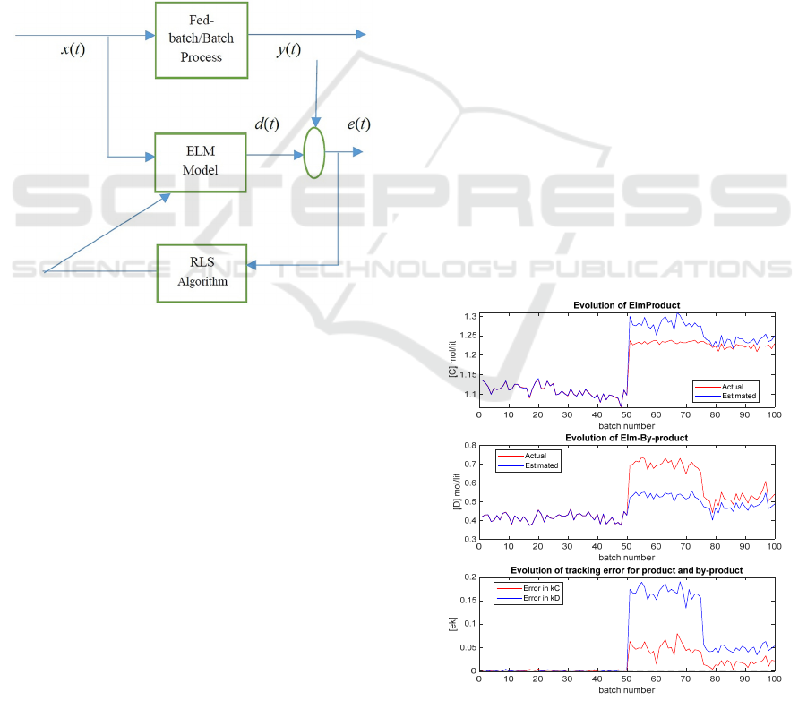
The schematic representation of the proposed
method is illustrated in Figure 1 below:
Figure 1: Integrating ELM with RLS.
Both fed batch and batch processes are vital mode
of process operation commonly used in many
chemical and pharmaceutical manufacturing
industries. In these process operations, the interest
lies in the final-batch product quality. To obtain an
optimal control policy for the process operation,
model capable of predicting accurate final predictions
(i.e. batch-end) is required. Therefore, data-driven
model is sought to overcome the problem of model
mismatch.
However, ELM model prediction does produce
good approximation of long-range model for
nonlinear batch processes but due to inadequate
historical process data and inaccuracy in data quality
used, model mismatches are inevitable when used on
real plant process operation which call for merging the
RLS technique with the ELM model predictions. A
stepwise description of the steady state proposed
modelling of the case study is as follows:
Step1: Collect N (e.g. N = 50) batches of historical
process operation data to develop an ELM model.
In this work, the historical process operation data
are generated through simulation. In the
simulation, piece-wise constant feeding profile is
used. The batch time (120 minutes) is divided into
10 equal intervals of 12 minutes and the feed rate
is constant during an interval with the constraint
00.1.
Step 2: Run the ELM modelling procedure to obtain
the output weights.
Step 3: Initialize the parameter estimation of the RLS
technique with the predicted output weights
obtained from the ELM and
(
)
=(0).
Step 4: Calculate the error between desired product
and the predicted product at each batch of the
iterations of the for-loop function.
Step 5: Calculate the Kalman gain with equation (14).
Step 6: Update the weights estimation with equation
(13).
Step 7: Update the
(
)
to
(
+1
)
at subsequent
iterations using equation (15).
5 SIMULATION RESULTS
This section presents the simulation results obtained
for modelling an isothermal fed-batch reactor
described in Section 2. It shows the comparison result
plots obtained for modelling with original ELM
method and plots for proposed method.
Figure 2: Plots of [C], [D] and [e
k
] under the ELM model.
ICAART 2020 - 12th International Conference on Agents and Artificial Intelligence
672
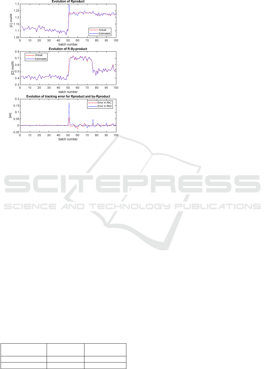
Figure3: Plots of [C], [D] and [e
k
] under the integrated ELM
and RLS model.
Figures 2 and 3 show the results obtained for the
conventional ELM model and the proposed integrated
ELM and RLS model respectively. In these figures,
an unknown disturbance is introduced from the 51
st
batch. In Figure 2, the first and the second plots show
the actual output /target data and the ELM predictions
for both [C] and [D] while the third plot shows the
prediction errors. Likewise, same plots are shown in
Figure 3 but with new proposed method. It can be
seen that the conventional ELM can model the first
50 batches well. However, after the presence of the
unknown disturbance, the prediction errors become
quite large. In contrast, the proposed ELM integrated
with RLS can adapt to the process changes and model
the process well after the presence of the unknown
disturbance.
Table 1 shows the values of the sum of square
errors (SSE) for predicting both [C] and [D] with the
conventional ELM and the proposed method.
The
SSE for the actual [C] is 0.3419 and [D] is 0.0689.
From Table 1, it can be seen that the proposed new
method modelled better and even from the figures
plots (i.e. Fig 2 and 3) shown above.
Table 1: Values of SSE for [C] and [D] under the ELM
model and the integrated ELM and RLS model.
Algorithm
methods
SSE for [C] SSE for [D]
ELM 0.3518 0.3425
ELM with RLS 0.0681 0.0531
6 CONCLUSIONS
An adaptive batch to batch modelling approach
integrating ELM with RLS for modelling fed-batch
processes is proposed in this paper. Through batch to
batch adaptation of ELM output layer weights, the
ELM model can track unknown disturbances and
process drift. Such a model is very useful in batch to
batch optimal control. Based on the results obtained
and comparison between the original ELM and the
proposed method, the proposed method showed better
modelling performance of the isothermal fed-batch
reactor process compared to the ordinary ELM.
Further research work will be done on batch to batch
optimisation control using the proposed modelling
method.
ACKNOWLEDGEMENTS
I would like to use this medium to appreciate the
effort of Petroleum Technology Development Fund
(Nigeria) for providing PhD scholarship to carry out
this research work successfully.
REFERENCES
Bonvin, D. (1998) ‘Optimal operation of batch reactors: a
personal view’, Journal of Process Control, 8, 355-368.
Chen, S., Billings, S.A. and Grant, P.M. (1990) 'Non-linear
system identification using neural networks',
International Journal of Control, 51(6), pp. 1191-1214.
Chi Sing, L., Kwok Wo, W., Pui Fai, S. and Lai Wan, C.
(1996) 'On-line training and pruning for recursive least
square algorithms', Electronics Letters, 32(23), pp.
2152-2153.
Huang, G.-B., Zhu, Q.-Y. and Siew, C.-K. (2006) 'Extreme
learning machine: Theory and applications',
Neurocomputing, 70(1), pp. 489-501.
Huang, G., Huang, G.-B., Song, S. and You, K. (2015)
'Trends in extreme learning machines: A review',
Neural Networks, 61(Supplement C), pp. 32-48.
Li, F., Zhang, J., Oko, E. and Wang, M. (2017) 'Modelling
of a post-combustion CO2 capture process using
extreme learning machine', International Journal of
Coal Science & Technology, 4(1), pp. 33-40.
Ruppen, D., Benthack, C., and Bonvin, D. (1995).
'Optimization of batch reactror operation under
parametric uncertainty – computational aspects',
Journal of Process Control, 5, 235-240.
Terwiesch, P., Ravemark, D., Schenker, B. and Rippin, D.
W. T. (1998) 'Semi-batch process optimization under
uncertainty: Theory and experiments', Computers &
Chemical Engineering, 22, 201-213.
Adaptive Modelling of Fed-batch Processes with Extreme Learning Machine and Recursive Least Square Technique
673

Wang, Y., Cao, F. and Yuan, Y. (2011) 'A study on
effectiveness of extreme learning machine',
Neurocomputing, 74(16), pp. 2483-2490.
Wigren, T. (1993) 'Recursive prediction error identification
using the nonlinear wiener model', Automatica, 29(4),
pp. 1011-1025.
Xiong, Z. and Zhang, J. (2005) 'A batch-to-batch iterative
optimal control strategy based on recurrent neural
network models', Journal of Process Control, 15(1), pp.
11-21.
Zhang, J. Morris, A. J., Martin, E. B. and Kiparissides, C.
(1999) 'Estimation of impurity and fouling in batch
polymerisation reactors through the application of
neural networks', Computers & Chemical Engineering,
23(3), 301-314.
ICAART 2020 - 12th International Conference on Agents and Artificial Intelligence
674
