A New Hybrid Salp Swarm-simulated Annealing Algorithm

for the Container Stacking Problem

Mohamed ElWakil

, Mohamed Gheith

1,2 b

and Amr Eltawil

Department of Industrial and Manufacturing Engineering, School of Innovative Design Engineering,

Egypt-Japan University of Science and Technology (E-JUST), Egypt

Faculty of Engineering, Alexandria University, Egypt

Keywords: Salp Swarm Algorithm, Container Terminals, Container Stacking Problem, Simulated Annealing.

Abstract: In container terminals, the shipping containers are stored temporarily in yards in the form of bays composed

of vertical stacks and horizontal rows. When there is a need to retrieve a target container, it may not be located

on the top of its stack, in such a case, the containers above it are called blocking containers. These blocking

containers should be relocated first in order to retrieve the target container. These relocations introduce an

extra workload and a challenge to the container terminal efficiency. In the Container Stacking Problem (CSP),

a group of containers are to be stacked in a given bay, while considering the future retrieval of these containers

with minimum number of relocations. In this paper, a new hybrid Salp Swarm-Simulated Annealing

Algorithm (SSSA) is proposed for solving the NP hard CSP. The contributions of this paper are as follows,

first, and for the first time, a discrete optimization version of the Salp Swarm Algorithm (SSA) is proposed.

The algorithm is different from the original continuous optimization one. Second, the SSA performance is

enhanced with a simulated annealing algorithm to improve its exploration capability. In order to examine the

performance of the proposed algorithm, computational experiments were performed on benchmark instances

that illustrated the competitive performance of the SSSA with respect to the optimal solutions of the instances.

1 INTRODUCTION

The global seaborne trade was about 11 billion tons

in 2018 and expected to increase at an average annual

growth rate of 3.5 per cent over the 2019–2024

period, (UNCTAD 2019). In 2018, a total of 793

million TEUs were handled in container ports around

the world. The increase in the number of containers

handled annually will need more efficient CTs that

can accommodate these high workloads. As CTs have

limited infrastructure, the high workloads will take

from the CT efficiency (Deng 2013).

A container terminal has three main areas; the

quay side, the yard side, and the land side. Containers

are stored in the yard side, coming from either the

quay side or the land side. Containers are stacked

above each other, forming blocks, each block has a

set of bays, each bay has a set of stacks and each stack

consists of a set of rows. The intersection between a

https://orcid.org/0000-0002-6066-6547

https://orcid.org/0000-0003-2092-2697

https://orcid.org/0000-0001-6073-8240

stack and a row results in a slot. A slot can hold only

one container. Each container in the yard area has a

designated slot to be stored in (Gheith et al., 2014a).

One of the performance measures of the CTs is the

container dwell time. It is the time that the import

container – as an example – spent at the CT starting

from the vessel’s arrival time to unload the container

and ending with the departure time of the External

Truck (ET) carrying the container out of the CT. CTs

always aim to minimize this dwell time to receive

more containers to gain more profits (Merckx, 2005).

Between the vessel unloading and external trucks

loading processes, the import containers are stored

temporarily in the CT’s yard. The CT’s yard receives

the unloaded containers from the vessels ordered by

their unloading sequence. Each container’s waiting

time is affected by the arrival time of the ET which

will deliver this container to the customer. Such

pickups are recently scheduled using Truck

Appointment Systems (TAS) (Azab et al 2017).

ElWakil, M., Gheith, M. and Eltawil, A.

A New Hybrid Salp Swarm-simulated Annealing Algorithm for the Container Stacking Problem.

DOI: 10.5220/0008974700890099

In Proceedings of the 9th International Conference on Operations Research and Enterprise Systems (ICORES 2020), pages 89-99

ISBN: 978-989-758-396-4; ISSN: 2184-4372

When a Target Container (TC) is scheduled to be

retrieved and it is not stored at the top of its stack, the

containers above it are called Blocking Containers

(BCs). These BCs need to be relocated first to retrieve

the target container. These relocations increase the

dwell time of the container. As relocations are time

consuming movements in CTs, they must be

minimized (ElWakil et al 2019).

One of the methods to minimize the relocations is

to initially store the containers while considering their

pickup orders. This will result in a better space

utilization and decrease containers dwell times (Böse,

2011). Thus, in the Container Stacking Problem (CSP)

a group of containers are to be stacked in a given bay

while considering the future retrieval of these

containers with minimum number of relocations. The

input of the CSP is the retrieval sequence of containers

from the vessel, in addition to the pickup sequence of

these containers from the yard which is provided by the

TAS. Whilst, the output will be the staking position of

each container in the bay (i.e. bay layout).

In this paper, a new Salp Swarm Algorithm is

proposed for discrete optimization problems. Then,

hybridization of this new version with Simulated

Annealing is proposed for solving the CSP. The new

hybrid algorithm is called the “Salp Swarm-

Simulated Annealing Algorithm” (SSSAA). The

algorithm performance was tested, and its results

were compared with optimal solutions of benchmark

instances from the literature.

2 RELATED WORK

The CT is an aggregate of container handling

operational processes, where all processes are

interconnected. Steeken et al., 2004 outlined these

operations while Schwarze et al., 2012 presented the

operations’ principles. The largest portion of these

processes is performed in the yard area. It is the main

storage area for containers in the CT (Covic, 2018).

Considering the yard area operations, three main

types of problems exist. The objective of them is to

increase the yard area productivity by minimizing the

number of relocations during pickups. However, the

method for achieving this objective is different for

each type. Formally, the three types are:

1. Stacking problems; they deal with the initial

storage of containers in the yard area (Zhang et

al., 2003; Dekker et al., 2007)

2. Relocation problems; they are dynamic

optimization problems which aim to find the

minimum number of relocations while

retrieving a set of containers (Forster and

Bortfeldt, 2012; Tang et al., 2015; Covic,

2017).

3. Marshalling problems: they are searching for

the optimal sequence of movements to be

performed on BCs to pickup a TC. (Lee and

Hsu, 2007; Caserta et al., 2012; Gheith et al.,

2014b; ElWakil et al., 2019).

The container stacking problem (CSP) is an

optimization problem that belongs to type one. The

CSP is to assign slots to the incoming containers such

that the number of future relocations is minimized.

The CSP is solved optimally by exact methods

(cf. e.g., Lehnfeld and Knust, 2014) or by heuristic

methods. In this paper, the literature review is limited

to the heuristics developed for solving the CSP.

Kim and Park, 2003 proposed two heuristics to

solve the CSP after proposing a formulated mixed

integer programming model for the problem.

Genetic Algorithms (GA) were used to solve the

CSP (Preston and Kozan, 2001; Bazzazi, 2009; Park

and Seo, 2009). Whilst, a simulation model based on

a genetic algorithm was proposed by Sriphrabu et al.,

2013. The aim was to find the best bay layout to

minimize the lifting time. A Tabu Search (TS)

algorithm and a hybrid algorithm between TS and GA

was proposed by Kozan and Preston, 2006 to solve

the problem. Park et al., 2011 developed an online

search algorithm to optimize the stacking policy in an

automated terminal. They also introduced a set of

criteria that must be considered to obtain a good

stacking position for each incoming container.

Chen and Lu, 2012 proposed for the CSP a Hybrid

Sequence Stacking Algorithm (HSSA) that determines

the exact location for each individual container upon

its arrival at the terminal. HSSA proved to be better

than random stacking algorithm and vertical stacking

algorithm. Moussi et al., 2012 proposed a hybrid

genetic simulated annealing algorithm to solve the

CSP. Ndiaye et al., 2014 proposed a hybrid ant colony-

bee algorithm to solve the CSP.

Gharehgozli et al., 2014 developed a decision-tree

heuristic that was efficient for the small-scale CSP

problems where the dynamic programming was used

for solving the large-scale ones. Hu et al., 2014 used

an outer-inner cellular automaton method to solve the

problem of choosing a certain bay and stacking

containers in this bay. The two problems were used

as an integrated optimization process.

Guerra-Olivares et al., 2015 proposed a Smart

Relocation (SR) heuristic to stack the outbound

containers in the yard considering the number of

relocations. Rekik et al., 2018 proposed a case-based

heuristic for the online container stacking

management system in seaport terminals. This

ICORES 2020 - 9th International Conference on Operations Research and Enterprise Systems

heuristic is sensitive to unexpected issues or

disturbances. Rekik and Elkosantini, 2019 proposed a

container terminal operating system that can capture,

store and reuse knowledge to detect disturbances for

selecting the most appropriate storage strategy and

determine the most suitable container location.

He et al., 2019 solved the CSP with a particle

swarm optimization algorithm. They applied the

neighbourhood-based mutation operator and

intermediate disturbance strategy to enhance the

exploration of the algorithm.

Boge and Knust 2020 discussed the CSP from a

general point of view as what so called the parallel

stack loading problem considering different fitness

functions. They first introduced a mixed integer

programming modelling of the problem adapted from

Boysen and Emde 2016. Then they presented a new

MIP model and a simulated annealing algorithm for

minimizing the total number of reshuffles in the

unloading stage.

This paper focuses on solving the CSP for

minimizing the future relocation to empty a bay. The

CSP is a combinatorial optimization problem with NP

hard nature (Bruns et al., 2016). So, the Salp Swarm

Algorithm (SSA) (Mirjalili et al., 2017) was adopted

to get better solutions for this problem. SSA is a

relatively new metaheuristic. It has been successfully

applied to solve such a combinatorial optimization

problem and has been proved to have an efficient

performance (Elkassas and ElWakil, 2019). SSA

hasn’t been applied for solving any kind of the CT

optimization problem yet.

Although, SSA has good convergence rate, but

there are still some disadvantages, such as the fall into

local optima and exploitation propensity (Sayed et al.,

2018). Hybridization of nature-inspired algorithms is

a popular approach to merge merits and strength of

standalone algorithms for handling those deficiencies

(Cheng and Prayogo, 2014). So, this paper proposes

a new hybrid salp swarm-simulated annealing

algorithm for solving the CSP.

3 THE CONTAINER STACKING

PROBLEM

In the container stacking problem (CSP), a set of

containers is to be stacked into a bay, for minimizing

the number of future relocations needed to empty this

bay. In other words, it is the problem of assigning the

proper slot for each container with the objective of

minimizing the number of future relocations needed

to empty the bay. The arrival sequence of the

containers to the bay and the retrieval sequence of the

containers from the bay is known in advance.

Each group of containers is represented by a set 

consists of number of  containers where 





,



,…,



. Each container takes a value of





which provide two-necessary information; the

value of 



defines the container’s pickup order, and

the position of 



in the set represent the container’s

arrival sequence to the bay. As an example, if 

2,5,9,1,8,6,7,3,4, then the first container

that will be retrieved is the fourth arrived container,

while the last to be retrieved is the third arrived one.

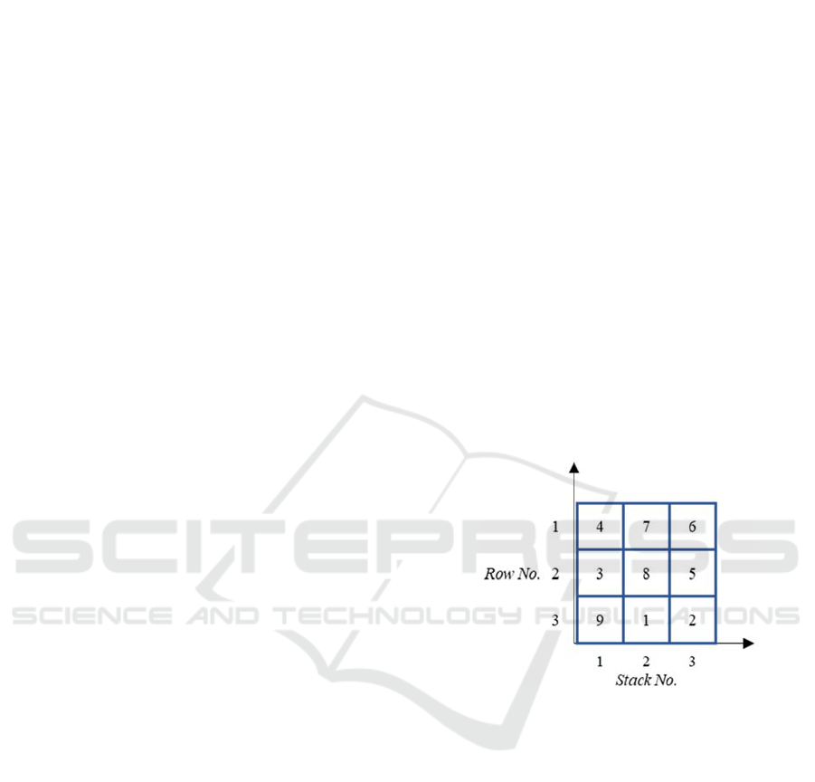
A bay consists of vertical stacks numbered by

1,2,…,



, and horizontal rows 1,2,…,



. A bay

layout  is shown in Fig. 1 of the containers in

set . Any  generated for  has a feasibility

condition that must be met. The condition is that any

incoming container can’t be stacked beneath its

predecessor. Formally, the feasibility condition can

be stated as: for any two containers 



,



∈, if 

 then 













, where  is the row number

of container .

Figure 1: A representation of a bay layout.

In the proposed method for the CSP, a solution of

a given set  is to specify a stack for each container

and the containers belonging to the same stack will be

stored according to their arrival sequence (the

feasibility condition). Formally, the solution is











,









,









,…,









. So, for the

bay layout  shown in Fig. 1, the solution is









3,3,1,2,2,3,2,1,1



. For sure, any solution

would be infeasible if the number of containers

assigned to specific stack exceeds the number of rows

in the bay. The bay layout  is equivalent to 



and provides a more obvious form for evaluating





. Each  has only one  whereas the feasibility

condition is held.

During pickups, Last-In-First-Out policy is

applied. So, if the TC is not on the top of its stack, all

the BCs must be relocated prior to picking up the TC.

A New Hybrid Salp Swarm-simulated Annealing Algorithm for the Container Stacking Problem

These relocations are unproductive moves and should

be minimized. Therefore, to evaluate any 

considering the number of blocking containers and

number of relocations, the following criteria have

been proposed:

 : Number of unordered pairs in all stacks.

Every couple of adjacent containers in a stack

is considered unordered if the upper container

is blocking the other one (Boysen and Emde,

2016; Lehnfeld and Knust, 2014).

 : Number of badly placed containers. A

container is considered badly placed if it blocks

the container below it through all the stack not

only the adjacent one (Bacci et al., 2017; Boge

and Knust, 2020).

 : total number of relocations needed to

empty the bay, according to their pickup order.

It considers the relocations only and excludes

the retrieval ones (Ndiaye et al., 2014).

If the bay layout  in Fig. 1 is considered, the

values of the 







is 4 (container 4, 8, 6 and 5),

whilst the 







is 5 (container 4, 7, 8, 6 and 5). In

this paper, only the  measure is considered.

So, formally the CSP can be described as: Find

 for a given set , so that 









minimum. Where, 



∗



4 THE PROPOSED APPROACH

The proposed approach is based on hybridization

between the Salp Swarm Algorithm (SSA) and the

Simulated Annealing (SA) algorithm to solve the CSP.

As the CSP is a discrete optimization problem, a new

version of the SSA is proposed for solving the discrete

optimization problems. To the best of our knowledge,

there is no reference to a discrete optimization version

of the SSA in current literature. Before presenting the

proposed approach, a brief about each of the

algorithms will be presented first, then the reason for

why hybridizing both algorithms is explained. Finally,

the proposed approach is presented.

4.1 Motivation of the Proposed

Approach

Although SSA has been proved to solve optimization

problems efficiently in comparison with other

metaheuristics, but in most cases, it is trapped in local

optima (Sayed et al., 2018). Therefore, to overcome this

challenge and enhance the SSA performance, a new

hybrid algorithm called hybrid salp swarm-simulated

annealing algorithm is proposed to solve the CSP.

During this work SA controls the acceptance of

bad generated leaders through the discrete version of

the SSA. By this hybridization, a balance between

exploration done by the followers and exploitation by

the leader is achieved without trapping the leader and

the swarm into the local optima. The performance of

the proposed algorithm for solving the CSP has been

assessed by benchmark instances from the literature.

Experimental results illustrate that the proposed

algorithm is efficient and robust for the CSP.

4.2 Salp Swarm Algorithm

4.2.1 Salp Swarm Algorithm for Continuous

Optimization

Salp Swarm Algorithm (SSA) has been proposed

recently by a biological inspiration of the salp’s food

search mission in deep seas (Mirjalili et al., 2017). It

is developed mainly for solving continuous

optimization problems. SSA showed a good and

robust converging to the optimum solution. The

concept of the leader and followers are the main idea

of the SSA performance (Fig. 2) (Mirjalili et al.,

2017). The leader is the best agent of the swarm and

it is the first salp in the swarm chain. The leader salp

is updated with respect to the food source (the best

solution ever found). The leader guides the swarm as

every follower follows its superior (the adjacent

preceding salp) (Mirjalili et al., 2017).

(a) (b)

Figure 2: (a) a salp agent (b) swarm of salps.

Every salp agent  is a candidate solution to the

optimization problem. So, the salp’s size (number of

dimensions) is equal to the number of variables

needed to be optimized. So, if the swarm consists of

 salps where every salp has  dimensions, 





the 



dimension of the 



salp, where  and

.

The SSA algorithm can be summarized as

follows: Initially, a number of  salps are generated

randomly and evaluated based on the evaluation

criteria of the solution. The salp with the best fitness

Leader

ICORES 2020 - 9th International Conference on Operations Research and Enterprise Systems

after evaluation is promoted to be the leader 



. The

food source  is the stored value of the best salp (i.e.

solution) ever found. So, in the beginning, it takes the

value of the leader salp.

Then, until reaching the termination condition, the

swarm is updated using numerical equations. As

stated earlier, the leader salp agent is updated with

respect to the food source . Equation (1) is used for

updating the leader position.

































,



0.5

























,



0.5



(1)

The exploration effectiveness of the SSA depends

mainly on the coefficient 



and it is generated in

each iteration by Equation (2), where  is the current

time and  is the maximum run time which after it the

algorithm stops. The value of 



decreases

exponentially with time leading to explore more

spaces at the beginning of the search and then limit

the search gradually iteration after iteration.

The upper and lower values for each dimension 

are represented as 



and 



respectively.

Parameters 



and 



control the search direction to

be balanced between both sides of the food source.

They are random number generated every iteration in

the interval [0, 1].





2















(2)

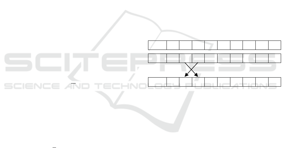
The followers are updated using Newton’s law of

motion. Equation (3) updates the value of each

follower agent, where 2. The new follower salp

value will be as the halfway between the new superior

salp agent 



and the old salp agent.

́





















(3)

After each iteration, the food source is updated

when a new better solution is found. At the end the,

the food source value is returned as the best solution.

4.1.2 Salp Swarm Algorithm for Discrete

Optimization

In SSA, Equation (1) and (3) are responsible for

updating the leader and the follower agents. These

two equations can be applied to continuous

optimization problems only when the values of

solutions are continuous numbers.

As stated earlier, the solution of CSP is an

assignment of each container ∈ to a stack ∈

1,2,…,



 satisfying that 













where





 is the number of occurrences of stack  in

.

The CSP is a Combinatorial Optimization

Problem (COP). Considering Fig. 1, a solution 



associated with the problem input  is illustrated

again in Fig. 3. A new solution 





can be generated

by swapping any two stacks’ positions which means

assigning new two stacks to the corresponding two

containers. As an example, 





means that 





1

and 





3instead of 





3 and 





1 in

the previous solution 



In the original SSA, Equation (1) updates the

leader salp 



to search around the food source .

The coefficient 



guarantees the random search

around the food source  while the coefficient 



determine how far the leader salp 



go from the food

source  to find new solutions (i.e. exploration). The

coefficient 



balances the search direction to

positive infinity or negative infinity which has no

meaning for COP.

 2 5 9 1 8 6 7 3 4





3 3 1 2 2 3 2 1 1







3 1 3 2 2 3 2 1 1

Figure 3: a representation of CSP solutions with its input .

Considering any COP generally, a new strategy is

proposed to update the leader salp agent with respect

to the food source instead of Equation (1).

Leader Update

Strategy (LUS)

Update 



by performing a

number of 



pair swap of any

two random dimensions of the

food source .

By using LUS, the same concept of updating the

leader salp 



is preserved. The coefficient 



is the

same while 



is represented in the LUS by the

random pair selected for the pair swap process.

However, based on trial experiments, a

modification to Equation (1) is performed and 



will

be updated according to Equation (4). Equation (4) is

plotted in Fig. 4 for a value of 30. Fig. 4 depicts

that Equation (4) allows the SSA to expand its search

space gradually until reaching a maximum value in

about the third of the maximum time. Then, it

A New Hybrid Salp Swarm-simulated Annealing Algorithm for the Container Stacking Problem

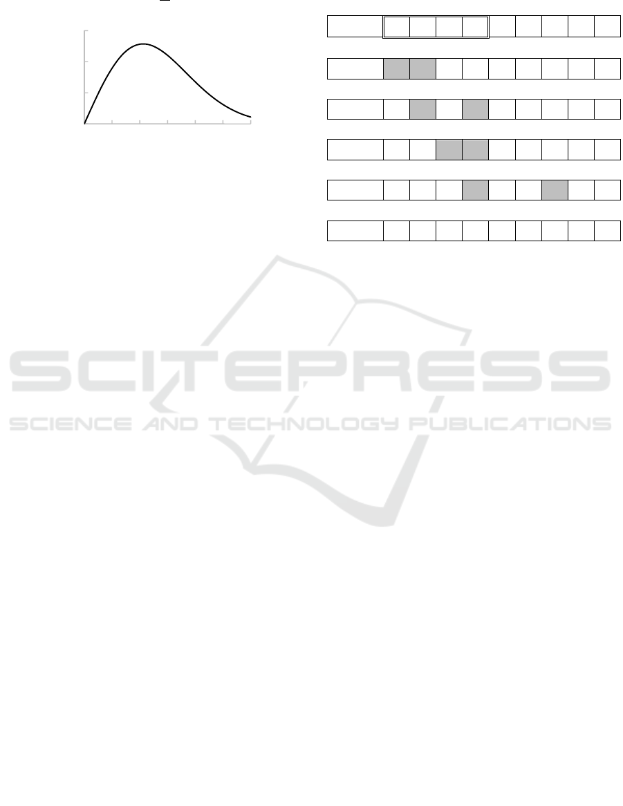
intensifies the search space be limiting the search

space gradually until the end.





2













(4)

Figure 4: Plot of Equation 4 for 30.

After performing a number of 



random pair

swaps on the food source , a new leader salp is

generated. Also, a number of 



1 new salps are

generated through the updating process. As every pair

swap performed, a new salp will be generated until

performing all the 



pair swaps.

In this paper, during updating the leader salp, the

evaluation of each generated salp is considered. If any

generated salp is better than the old leader, it is

assigned as a new leader salp on the spot and the

updating process is completed by updating this new

leader salp.

For updating the follower salps, a new strategy is

also proposed producing the same effect that

Equation (3) does.

For any two salps with  size, one of them can be

transformed into the other by performing at most 

pair swaps. This is applicable since the constituents

of the salp (i.e. number of stacks repeated 



times)

are the same, the only change will be the assignment

of these stacks to containers.

Equation (3) generates the new follower salp ́



by taking the average of the values of its new superior





salp and the old follower salp 



. The follower

update strategy (FUS) suggests performing half of the

pair swaps needed to move from the old 



to the new





Follower Update

Strategy (FUS)

Update 



by performing

half of the pair swaps to

move from the old salp to the

new superior salp.

Fig. 5 illustrate the follower update strategy

(FUS). The target is to move half the way from the

old salp 



to the new superior salp 



. So, the first

half of the old salp 



is considered to have pair swaps

to generate the first half of the new superior salp 



In each step, the necessary pair swap is filled with

grey.





3 2 1 2 2 1 3 1 3





1 3 3 2 2 3 2 1 2

⇩

1 3 2 2 3 2 1 2

⇩

3 2

3 1 2 3 2 1 2

⇩

3 2 1

3 1 1 2 1 2

⇩





3 2 1 2 3 3 2 1 2

Figure 5: Illustration of the FUS.

The original SSA is accepting the new generating

salps (leader and follower) even the solution is not

improved.

In this paper, the generated salps will be accepted

even if they are not better solutions except the leader.

The leader is replaced only by a better salp generated

from updating any salp of the swarm. Trail

experiments showed that accepting bad leader salp

directs the swarm away from the food source even

with updating the leader with respect to the food

source. Also, accepting bad followers can’t be

abandoned for investigating the way from the old

search space to the new one through iterations.

By using this approach, the acceleration of the

SSA is increased by updating rapidly the leader salp.

And that will direct all the swarm to the global

optima. Accepting the new generated follower salps

increase the exploration range for the swarm, but that

was not enough to escape from the local optima. That

was solved using the SA.

4.2 Simulated Annealing

Simulated Annealing (SA) is a powerful

metaheuristic that used for solving large COPs based

on the simulation of the annealing of solids process

(Van Laarhoven and Aarts, 1987).

The basic idea of SA is to accept bad solutions at

the beginning of the search by a given probability,

which may lead to better solutions after a while. This

acceptance probability decreases with time utilizing

the concept of solids cooling during annealing

process. The temperature value







controls the

0 5 10 15 20 25 30

ICORES 2020 - 9th International Conference on Operations Research and Enterprise Systems

acceptance probability of bad solutions during the

search process as in Equation (5), where Δ is the

difference between the finesses of the considered

solutions.







∆





(5)

At the beginning of the search process, a higher

relatively temperature value is assigned. This initial

temperature 



is reduced by the so called

“cooling procedure” through every cooling step. The

cooling procedure is executed by Equation (6), where

 is the cooling factor. The temperature is reduced

after a number of  iterations.

∗

(6)

A reheating process may be needed. If the

temperature value drops below a specific value 



the temperature is set to its initial value (Hussin and

Stützle, 2014).

4.3 The Proposed SSSAA Algorithm

New hybrids of the existing algorithms are being

developed to solve different optimization problems.

In this paper, our new version of the salp swarm

algorithm for COPs is hybridized with the simulated

annealing algorithm. It is called by SSSAA which

merges the salp swarm algorithm (SSA) with the

simulated annealing (SA) for updating the leader salp

only. Further, the new hybrid algorithm is detailed as

follows:

Step 1: Population Initialization.

A population of a number of  salps is

randomly generated. Each salp 



is a random vector

of  dimensions. For the CSP, the values of the salp

are a random assignment of bay stacks to the

containers of .

Step 2: Evaluation.

Every salp is evaluated based on the fitness

function used for the problem. For the CSP, the

fitness of every salp is measured by 









explained earlier. The swarm is sorted and the salp

with the best fitness function so far is assigned to

be the leader salp and the rest are followers with

descending superiority. The food source is

assigned as the best salp ever found. At the end of

this step, the leader salp’s value is stored.

Step 3: Main Loop.

The main loop is started after the initialization and

evaluation steps. It begins with defining the food

source  as the best salp found through the

execution. After that, the salp swarm is updated until

reaching the stopping condition.

Step 4: Updating the Leader Salp.

All the salps are updated at each iteration through

the main loop. The leader salp 



 is updated with

respect to the food source . The 



 coefficient

value is calculated first using Equation (4). Then, the

LUS is used.

The LUS performs a number of pair swaps equal

to 



. After each pair swap a new leader salp is

generated. The corresponding fitness function of this

new leader salp is evaluated. This new leader salp is

accepted instantly if it has a lower fitness value than

the previous one. If it hasn’t, it is rejected or accepted

based on the SA probability. A leader with higher

fitness is accepted as a new leader salp not a food

source  of course. This evaluation and accepting or

not process is repeated until all the 



pair swaps is

finished.

Step 5: Updating the Follower Salps.

Each follower salp is updated with respect to its

superior. The updated follower salp 



 is

generated from the old value follower salp 



 by

performing the FUS with respect to the its new

superior 



 where 2.

Step 6: Stopping Condition.

The main loop is repeated updating the swarm

based on Step 3 and 4 until the time of execution

exceed the value of . is set to equal to the 

seconds (i.e. number of containers). So, if an instance

has a dimension of 30 containers, the algorithm will

stop after 30 seconds. The food source is returned as

the best solution found for the problem.

All the parameters’ values of SSSAA are

summarized in Table 1.

Table 1: SSSAA parameters’ values.

Parameter Value







0.01



100



0.9

A New Hybrid Salp Swarm-simulated Annealing Algorithm for the Container Stacking Problem

The pseudo code of the SSSAA is as follows:

SSSAA

1: For 1:

2: 



stackingofcontainers

4: 









5: End

6: 



7: While 

8: 



withmin

9: 



min

10: Update 



with Equation (4)

11: For 1:

12: If 1

13: 1:



14: 



pairofstacks

15: new







afterswap



16: _







new





17: If _



< 



18: 



new



19: 



_



20: Else

21: Δ_



- 



22: Calculate with Equation (5)

23: If rand < 

24: 



new



25: 



_



26: End

27: End

28: 1

29: IF 100∗

30: 0

31: Update  with Equation (6)

32: IF 



33: 



34: End

35: End

36: End

37: Else

38: update 



using FLU

39: 









40: End

41: End

42: End

43: Return 

5 COMPUTATIONAL RESULTS

The SSSAA was coded using MATLAB 2017b and

was run on a PC equipped with an Intel(R) Core(TM)

i5-4200M CPU @ 2.5 GHz and 8 GB RAM under the

Windows 10 operating system.

To test the performance of the SSSAA, the set of

benchmark instances from Boge and Knust, 2020

were considered. They solved each instance with a

MIP formulation for the fitness function 

imposing a time limit of 30 minutes. They stated that

only some of these instances were solved to

optimality within the time limit.

The characteristics of the benchmark instances are

as shown in Table 2. The number of containers to be

stacked is , while 



and 



determine the size of the

target bay. When the bay isn’t filled completely with

the  containers i.e. 



∗



,  is marked with an

asterisk (∗). Each row in the table represents a group of

20 instances having the same characteristics. The

fourth column in the table defines the number of

instances that have been verified to be solved to

optimally out of the 20 instances according to Boge

and Knust, 2020. They also have reported the average

times of getting the optimal solution. For some of the

instances, the maximum of 30 minutes wasn’t enough

to reach the optimal solutions. The average fitness

function  and the average times in seconds of

each 20 instances are reported in the fifth columns. The

larger instances with 120 are discarded through

our experiments as practicality, the maximum bay

dimensions are 8 stacks with 6 rows corresponding to

the yard crane reachability (Gheith et al., 2016).

In the sixth column of Table 2, the results of the

new version of the SSA and the corresponding times

are reported. It is evident that the SSA results were so

far from the optimal solutions due to the reasons

stated earlier in section 4.

The SSSAA robust performance can be observed

from the results in the seventh column of Table 2. The

hybrid algorithm results are so close to the optimal

solutions. Hybridization of the new version of SSA

with SA has improved its performance. The average

times of the SSSAA is challenging for large instances

(60) and they may be considered high compared

to the MIP times especially for the small size instance

where∈30,40. As the average values can’t be

guaranteed as a performance measure, a second

evaluation may be needed.

The second evaluation was performed for the

individual instances of the same instance groups.

Table 3 reported the difference in the fitness function

value between the SSSAA value and the best value

reported by MIP in Boge and Knust, 2020. This

difference is underlined if it is more than zero.

Table 3 demonstrates the SSSAA capability of

finding the reported best solution for most of the

instances in a challenging time.

In Table 2, the MIP average times were lower than

the SSSAA ones especially for ∈30,40 .

However, there are some individual instances needed

times to be solved by MIP more than the SSSAA and

the resulted fitness function values  were the

same. Each such instance was highlighted by grey in

Table 3 illustrates that sometimes SSSAA can find

the same solutions produced by MIP but in less time.

ICORES 2020 - 9th International Conference on Operations Research and Enterprise Systems

Table 2: The average solutions’ UP fitness for SSSAA compared with optimal solutions.

 







Ver

MIP (Boge and

Knust, 2020)

SSA

SSSAA



time



time



time

30 5 6 20 4 1.4

5.30 30

30 6 5 20 2.9 0.1

5.00 30

2.95 30

∗30

8 4 20 1.05 0.1

3.15 30

1.1 30

30 10 3 20 0.4 9.9

1.50 30

0.4

40 5 8 20 4.9 0.2

7.55 40

4.9

∗40

7 6 20 2.7 0.4

5.9 40

2.75 40

40 8 5 20 1.8 2.5

5.25 40

1.95 40

40 10 4 20 0.75 254.0

3.4 40

0.85 40

60 6 10 20 6.8 0.9

11.4 60

7.15 60

60 10 6 18 2.4 183.8

8.85 60

3.25 60

60 12 5 13 1.05 664.3

7.95 60

1.6 60

60 15 4 11 0.5 811.5

4.85 60

0.8 60

60 20 3 17 0.15 270.9

1.35 60

0.15

Table 3: Performance of SSSAA for individual instances.

Instances group Difference between SSSAA and the optimal solution for every instance

 







1 2 3 4 5 6 7 8 9 10 11 12 13 14 15 16 17 18 19 20

30 5 6 0 0 0 0 0 0 0 0 0 0 0 0 0 0 0 0 0 0 0 0

30 6 5 0 0 0 0 0 0 0 0 0 0 0 1 0 0 0 0 0 0 0 0

∗30

8 4 0 0 0 0 1

0 0 0 0 0 0 0 0 0 0 0 0 0 0 0

30 10 3

0 0 0 0 0 0 0 0 0 0 0 0 0 0 0 0 0 0 0 0

40 5 8 0 0 0 0 0 0 0 0 0 0 0 0 0 0 0 0 0 0 0 0

∗40

7 6 0 0 0 0 0 1

0 0 0 0 0 0 0 0 0 0 0 0 0 0

40 8 5 0 0 0 0

0 1 0 0 1 0 0 0 1 0 0 0 0 0 0 0

40 10 4 0 0 0 0 0 1 0 0 0 0 0 0 0 0 0 1 0 0 0 0

60 6 10 0 0 0 0 1 0 0 1 0 0 1 1 1 1 0 1 0 0 0 0

60 10 6 0 1

1 0 1 1 1 1 1 1 0 2 1 1 1 1 1 1 0 1

60 12 5 0 0 1 0 1 0 0 1 0 1 0 0 2 1 1 0 0 1 1 1

60 15 4 0 0 0 0 0 0 1 1 1 0 0 0 0 1 1 0 1 0 0 0

60 20 3 0 0 0 0 0 0 0 0 0 0 0 0 0 0 0 0 0 0 0 0

A New Hybrid Salp Swarm-simulated Annealing Algorithm for the Container Stacking Problem

6 CONCLUSIONS

In this paper, a new version of the salp swarm

algorithm for discrete optimisation problems is

propose. Then it is hybridized to develop a new

hybrid salp swarm simulated annealing algorithm

(SSSAA). It integrated the simulated annealing (SA)

with the new version of the salp swarm algorithm

(SSA) for overcoming the local optima trapping. The

SA enhanced the exploitation while updating the

leader salp of the swarm. The SSSAA performance

was tested by comparison to the best reported

solutions of the container stacking problem (CSP). As

the CSP is an operational process, it needed to be

performed frequently in a relatively fast time. The

SSSAA was capable of finding the optimal solution

for most of the tested instances in a relatively very

short time with respect to the mixed integer

programming reported in the literature. The

computational results reveal that SSSAA is a very

fast, efficient and capable tool for the CSP.

REFERENCES

Azab, A., Karam, A., and Eltawil, A., 2017. Impact of

collaborative external truck scheduling on yard

efficiency in container terminals. In International

Conference on Operations Research and Enterprise

Systems, 105-128, Springer, Cham.

Bacci, T., Mattia, S., and Ventura, P., 2017. Some

complexity results for the minimum blocking items

problem. In International Conference on Optimization

and Decision Science (pp. 475-483). Springer, Cham.

Bazzazi, M., Safaei, N., and Javadian, N., 2009. A genetic

algorithm to solve the storage space allocation problem

in a container terminal. Computers & Industrial

Engineering, 56(1), 44-52.

Boge, S., and Knust, S., 2020. The parallel stack loading

problem minimizing the number of reshuffles in the

retrieval stage. European Journal of Operational

Research, 280(3), 940-952.

Böse, J. W., 2011. General considerations on container

terminal planning. In Handbook of terminal planning,

3-22, Springer, New York, NY.

Boysen, N., and Emde, S., 2016. The parallel stack loading

problem to minimize blockages. European Journal of

Operational Research, 249(2), 618-627.

Bruns, F., Knust, S., and Shakhlevich, N. V., 2016.

Complexity results for storage loading problems with

stacking constraints. European Journal of Operational

Research, 249(3), 1074-1081.

Caserta, M., Schwarze, S., and Voß, S., 2012. A

mathematical formulation and complexity

considerations for the blocks relocation problem.

European Journal of Operational Research, 219(1),

96-104.

Chen, L., and Lu, Z., 2012. The storage location assignment

problem for outbound containers in a maritime

terminal. International Journal of Production

Economics, 135(1), 73-80.

Cheng, M. Y., and Prayogo, D., 2014. Symbiotic organisms

search: a new metaheuristic optimization algorithm.

Computers & Structures, 139, 98-112.

Covic, F., 2017. Re-marshalling in automated container

yards with terminal appointment systems. Flexible

Services and Manufacturing Journal, 29(3-4), 433-503.

Covic, F., 2018. A literature review on container handling

in yard blocks. In International Conference on

Computational Logistics (pp. 139-167). Springer,

Cham.

Dekker, R., Voogd, P., and van Asperen, E., 2007.

Advanced methods for container stacking. In Container

terminals and cargo systems (pp. 131-154). Springer,

Berlin, Heidelberg.

Deng, T., 2013. Impacts of transport infrastructure on

productivity and economic growth: Recent advances

and research challenges. Transport Reviews, 33(6),

686-699.

Elkassas, A. M., and ElWakil, M., 2019. Facility Layout

Problem Using Salp Swarm Algorithm. In 2019 6th

International Conference on Control, Decision and

Information Technologies (CoDIT) (pp. 1859-1864).

IEEE.

ElWakil, M., Gheith, M., and Eltawil, A., 2019. A New

Simulated Annealing Based Method for the Container

Relocation Problem. In 2019 6th International

Conference on Control, Decision and Information

Technologies (CoDIT), (pp. 1432-1437). IEEE.

Forster, F., and Bortfeldt, A., 2012. A tree search procedure

for the container relocation problem. Computers &

Operations Research, 39(2), 299-309.

Gharehgozli, A. H., Yu, Y., de Koster, R., and Udding, J.

T., 2014. A decision-tree stacking heuristic minimising

the expected number of reshuffles at a container

terminal. International Journal of Production

Research, 52(9), 2592-2611.

Gheith, M. S., Eltawil, A. B., and Harraz, N. A., 2014a. A

rule-based heuristic procedure for the container pre-

marshalling problem. In 2014 IEEE International

Conference on Industrial Engineering and Engineering

Management (pp. 662-666). IEEE.

Gheith, M. S., Eltawil, A. B., and Harraz, N. A., 2014b. A

rule-based heuristic procedure for the container pre-

marshalling problem. In 2014 IEEE International

Conference on Industrial Engineering and Engineering

Management (pp. 662-666). IEEE.

Gheith, M., Eltawil, A. B., and Harraz, N. A., 2016. Solving

the container pre-marshalling problem using variable

length genetic algorithms. Engineering Optimization,

48(4), 687-705.

Guerra-Olivares, R., González-Ramírez, R. G., and Smith,

N. R., 2015. A heuristic procedure for the outbound

container relocation problem during export loading

operations. Mathematical Problems in Engineering.

He, Y., Wang, A., Su, H., and Wang, M. (2019). Particle

Swarm Optimization Using Neighborhood-Based

ICORES 2020 - 9th International Conference on Operations Research and Enterprise Systems

Mutation Operator and Intermediate Disturbance

Strategy for Outbound Container Storage Location

Assignment Problem. Mathematical Problems in

Engineering, 2019.

Hu, W., Wang, H., and Min, Z., 2014. A storage allocation

algorithm for outbound containers based on the outer–

inner cellular automaton. Information Sciences, 281,

147-171.

Hussin, M. S., and Stützle, T., 2014. Tabu search vs.

simulated annealing as a function of the size of

quadratic assignment problem instances. Computers &

operations research, 43, 286-291.

Kang, J., Oh, M. S., Ahn, E. Y., Ryu, K. R., and Kim, K.

H., 2006. Planning for intra-block remarshalling in a

container terminal. In International Conference on

Industrial, Engineering and Other Applications of

Applied Intelligent Systems (pp. 1211-1220). Springer,

Berlin, Heidelberg.

Kim, K. H., and Park, K. T., 2003. A note on a dynamic

space-allocation method for outbound containers.

European Journal of Operational Research, 148(1),

92-101.

Kozan, E., and Preston, P., 2006. Mathematical modelling

of container transfers and storage locations at seaport

terminals. OR Spectrum: Quantitative Approaches in

Management, 28(4), 519-537.

Lee, Y., and Hsu, N. Y., 2007. An optimization model for

the container pre-marshalling problem. Computers &

Operations Research, 34(11), 3295-3313.

Lehnfeld, J., and Knust, S., 2014. Loading, unloading and

premarshalling of stacks in storage areas: Survey and

classification. European Journal of Operational

Research, 239(2), 297-312.

Merckx, F., 2005. The issue of dwell time charges to

optimize container terminal capacity. In Proceedings

IAME 2005 Annual Conference, Limassol, Cyprus, 23-

25 June 2005.

Mirjalili, S., Gandomi, A. H., Mirjalili, S. Z., Saremi, S.,

Faris, H., and Mirjalili, S. M., 2017. Salp Swarm

Algorithm: A bio-inspired optimizer for engineering

design problems. Advances in Engineering Software,

114, 163-191.

Moussi, R., Ndiaye, N. F., and Yassine, A. (2012, March).

Hybrid genetic simulated annealing algorithm

(HGSAA) to solve storage container problem in port. In

Asian Conference on Intelligent Information and

Database Systems (pp. 301-310). Springer, Berlin,

Heidelberg.

Ndiaye, N. F., Yassine, A., and Diarrassouba, I., 2014.

Hybrid Algorithms to Solve the Container Stacking

Problem at Seaport. GSTF Journal of Mathematics,

Statistics & Operations Research, 2(2).

Park, C., and Seo, J., 2009. Mathematical modeling and

solving procedure of the planar storage location

assignment problem. Computers & Industrial

Engineering, 57(3), 1062-1071.

Park, T., Choe, R., Kim, Y. H., and Ryu, K. R. (2011).

Dynamic adjustment of container stacking policy in an

automated container terminal. International Journal of

Production Economics, 133(1), 385-392.

Preston, P., and Kozan, E., 2001. An approach to determine

storage locations of containers at seaport terminals.

Computers & Operations Research, 28(10), 983-995.

Rekik, I., and Elkosantini, S., 2019. A Multi Agent System

for the online Container Stacking in Seaport terminals.

Journal of Computational Science.

Rekik, I., Elkosantini, S., and Chabchoub, H., 2018. A case

based heuristic for container stacking in seaport

terminals. Advanced Engineering Informatics, 38, 658-

669.

Sayed, G. I., Khoriba, G., and Haggag, M. H, 2018. A novel

chaotic salp swarm algorithm for global optimization

and feature selection. Applied Intelligence, 48(10),

3462-3481.

Schwarze, S., Voß, S., Zhou, G., and Zhou, G., 2012.

Scientometric analysis of container terminals and ports

literature and interaction with publications on

distribution networks. In International Conference on

Computational Logistics, (pp. 33-52). Springer, Berlin,

Heidelberg.

Sriphrabu, P., Sethanan, K., and Arnonkijpanich, B., 2013.

A solution of the container stacking problem by genetic

algorithm. International Journal of Engineering and

Technology, 5(1), 45.

Steenken, D., Voß, S., and Stahlbock, R, 2004. Container

terminal operation and operations research-a

classification and literature review. OR spectrum,

26(1), 3-49.

Tang, L., Jiang, W., Liu, J., and Dong, Y., 2015. Research

into container reshuffling and stacking problems in

container terminal yards. IIE Transactions, 47(7), 751-

766.

UNCTAD/RMT, 2019. Review of Maritime Transport

2019, United Nations publications. New York.

Van Laarhoven, P. J., and Aarts, E. H., 1987. Simulated

annealing. In Simulated annealing: Theory and

applications, 7-15, Springer, Dordrecht.

Zhang, C., Liu, J., Wan, Y. W., Murty, K. G., and Linn, R.

J., 2003. Storage space allocation in container

terminals. Transportation Research Part B:

Methodological, 37(10), 883-903.

A New Hybrid Salp Swarm-simulated Annealing Algorithm for the Container Stacking Problem