Dynamic Assignment Vehicle Routing Problem with Generalised

Capacity and Unknown Workload

F. Phillipson

1 a

, S. E. de Koff

, C. R. van Ommeren

and H. J. Quak

1,2

Netherlands Organisation for Applied Scientiﬁc Research (TNO), Den Haag, The Netherlands

Breda University of Applied Sciences, Breda, The Netherlands

Keywords:

Parcel Distribution, Cross Docking, Assignment.

Abstract:

In this paper we present a modiﬁcation to the Dynamic Assignment Vehicle Routing Problem. This problem

arises in parcel to vehicle assignment where the destination of the parcels is not known up to the assignment

of the parcel to a delivering route. The assignment has to be done immediately without the possibility of

re-assignment afterwards. We extend the original problem with a generalisation of the deﬁnition of capacity,

with an unknown workload, unknown number of parcels per day, and a generalisation of the objective function.

This new problem is deﬁned and various methods are proposed to come to an efﬁcient solution method.

1 INTRODUCTION

In city logistics, the efﬁcient and effective transporta-

tion of goods in urban areas is important. For the

community as a whole however, taking into account

the negative effects on congestion, safety, and en-

vironment (Savelsbergh and Van Woensel, 2016) is

important. These aspects come together in consoli-

dation and transshipment on satellite locations with

cross docking, redistributing the incoming freight into

other, possibly smaller vehicles to serve customers.

This results in a 2-echelon distribution and vehicle

routing problem (2E-VRP), which are described in

the survey of (Cuda et al., 2015). The authors of this

survey consider strategic planning decisions, includ-

ing decisions concerning the infrastructure of the net-

work, and tactical planning decisions, including the

routing of freight through the network and the allo-

cation of customers to the intermediate facilities. At

the tactical level, the customer locations are consid-

ered known. This is not the case in most situations in

practice. There, a considerable part of the customer

locations is revealed late in the process. This brings

us in the ﬁeld of dynamic vehicle routing problems.

The review of Pillac et al. (Pillac et al., 2013)

gives an overview of dynamic vehicle routing prob-

lems. They make a separation of those problems be-

tween ‘static and dynamic’ on one axis and ‘deter-

ministic and stochastic’ on the other axis. This gives

https://orcid.org/0000-0003-4580-7521

four ﬁelds of research. In ﬁeld (1) ’static and deter-

ministic problems’, all input is known beforehand and

vehicle routes do not change once they are in exe-

cution, see for an overview of these classic vehicle

routing problems (VRPs) (Baldacci et al., 2007). In

ﬁeld (2), ‘Static and stochastic’, problems are charac-

terised by input partially known as random variables,

which realisations are only revealed during the exe-

cution of the routes, see for example (Bertsimas and

Simchi-Levi, 1996). Here also clustering techniques

for stochastic data can be used (Ngai et al., 2006).

In ﬁeld (3) ‘dynamic and deterministic’ problems,

part or all of the input is unknown and revealed

dynamically during the design or execution of the

routes. These problems are also called online VRP

problems (Bjelde et al., 2017; Jaillet and Wagner,

2008). Similarly, in the problems of ﬁeld (4), ‘dy-

namic and stochastic’ problems, a part or all of their

input unknown. The unknown information is revealed

dynamically during the execution of the routes, but in

contrast with the latter category, exploitable stochas-

tic knowledge is available on the dynamically re-

vealed information. See for a survey (Ritzinger et al.,

2016). In addition, methods based on anticipation can

be used (Ulmer et al., 2015).

In (Phillipson and De Koff, 2020) the Dynamic

Assignment Vehicle Routing Problem (DA-VRP) is

introduced. This is a ﬁeld (3) ‘dynamic deterministic’

VRP, however, the assignment of the parcels is done at

the same time the destination is revealed. This means

that the planning is done dynamically, but in contrast

Phillipson, F., E. de Koff, S., van Ommeren, C. and Quak, H.

Dynamic Assignment Vehicle Routing Problem with Generalised Capacity and Unknown Workload.

DOI: 10.5220/0008933703290335

In Proceedings of the 9th International Conference on Operations Research and Enterprise Systems (ICORES 2020), pages 329-335

ISBN: 978-989-758-396-4; ISSN: 2184-4372

329

to the common dynamic case, it is done in upfront,

where the route is not being executed yet, giving the

possibility to change the order per route, but not to

interchange between the routes. This problem relates

directly to the practice in parcel distribution. Often,

a satellite location where the incoming parcels have

to be distributed over a number of vehicles to deliver

them to the customers, has no, or a rather small, space

for storage. This means that the parcels have to be as-

signed directly, after unloading and scanning, to an

outgoing vehicle. There is no possibility to reassign

on a later moment in time. The parcels are delivered

to the assigned vehicle instantaneously. The destina-

tion of the parcels is not known on beforehand and is

revealed only at arrival at the satellite location.

In (Phillipson and De Koff, 2020) an approach is

presented to solve this problem. However, some as-

sumptions are made there that will be generalised in

this work. This generalisation will be on:

• the capacity of the routes: this is now not only

driven by the number of parcels, but also by the

(time) length of the tour. The tour cannot be

longer than a speciﬁc time t.

• the forecast: we do not longer know the exact

number of parcels to be distributed per day. In

some cases we assume we have some approximate

forecast using a seasonal or weekly pattern.

• the objective: the objective to be minimised is

no longer only the total distance of the tours in

kilometres, but a combination of this total dis-

tance (monetised by multiplying it with a price-

per-kilometre) and the costs (salary cost per hour)

of the driver. For this we will round the number of

hours per driver to a certain amount (7 or 8 hours)

to illustrate what happens when a driver can only

be hired for (almost) a whole day.

The remaining of this paper is organised as fol-

lows. First, in Section 2, we present the general

approach to come to a dynamic assignment of the

parcels to the routes. In Section 3, we elaborate on

the cases we use to show the performance of the vari-

ous approaches. Conclusions can be found in Section

2 METHOD

In this section we present an approach that can be used

to assign the parcels to the routes. In (Phillipson and

De Koff, 2020) two steps were distinguished:

1. Initial assignment of direction to routes;

2. Dynamic assignment of arriving parcels;

The ﬁrst step gives a potential direction to each of the

routes, or none if empty vehicles are used, by assign-

ing a base load, a certain region or some initial direc-

tion. The second step assigns directly the incoming

parcels to the routes. The uncertainty about the num-

ber of parcels per day will lead to two extra steps in

our approach:

1. Initial assignment of direction to routes;

2. Dynamic decision of daily ﬂeet size;

3. Dynamic assignment of arriving parcels;

4. Post-processing.

All steps will be discussed in more detail in the next

sections. In Section 2.3 solution techniques that are

used, are presented in more detail. After those steps

the load assigned to all routes is known and for each

route a regular TSP can be solved.

2.1 Assumptions and Notation

In a Dynamic Assignment Vehicle Routing Problem

(DA-VRP) k parcels arrive at a location in a speciﬁc

order. In that speciﬁc order, each of the parcels reveal

their destination and have to be assigned immediately

to one of the m (identical) vehicles, that will deliver

the parcel to its destination. Each parcel requires one

capacity unit of the vehicles and all vehicles have ca-

pacity C. When assigning the jth parcel, vehicle i can

only be regarded iff n

< C, where n

equals the load

of vehicle i at that current moment. No information

is known or used about the geographical location of

the client. Only a estimation of the total volume is

assumed, based on a similar day in the past.

2.2 Detailed Steps

We go into more detail on each of the four steps.

Step 1: Initial assignment of direction to vehicles. It is

helpful to give an initial direction or assignment of a

certain area to each of the routes. This is done in Step

1 of the approach, the initial assignment. We consider

two possible approaches:

1. Separation by dummy location - We perform a k-

Means clustering over all potential customers and

assign a dummy parcel, having as location one of

the cluster means, to each route. K-means clus-

tering (James et al., 2013) aims to partition obser-

vations into k clusters, in which each observation

belongs to the cluster with the nearest mean.

2. Total geographical separation - Again we perform

a (k-Means) clustering over all potential customer

locations (postal codes) and assign each of those

(postal codes) clusters to a route.

ICORES 2020 - 9th International Conference on Operations Research and Enterprise Systems

330

Step 2: Dynamic decision of daily ﬂeet size. In

(Phillipson and De Koff, 2020) the (exact) number

of parcels is known in advance and from that we can

compute the number of routes we need, given only

a capacity constraint on the number of parcels. How-

ever, now we don’t know the number of required vehi-

cles for two reasons. Firstly we don’t (exactly) know

the number of parcels per day and, secondly, we don’t

know the location of the parcels and thus we don’t

know the (time) lengths of the resulting routes. This

means that we have to decide on the number of routes,

somewhere before, during or after the assignment of

arriving parcels. We actually do all three: we start

with a certain number, add extra routes during the

sorting process and ﬁnally, we combine, where pos-

sible, routes into one route after sorting. This also

means that Step 2 and Step 3 are happening some-

what in parallel: the number of tours are not deﬁned

beforehand but during the assignment. For the sake

of clarity, we will use the term tour for the ﬁrst three

steps. The result of the third step will then be a num-

ber of tours with parcels assigned to it. In Step 4 the

tours will be assigned to routes, that can be executed

by vehicles.

In Step 2 we decide on the number of tours to start

with, and on the procedure and conditions to add an

extra tour to the problem. We looked at two possible

approaches for this step. For both approaches we as-

sume a (rough) estimation of the number of arriving

parcels, coming from a seasonal or weekly pattern.

We estimate the number of tours to distribute these

parcels and call this number N for a certain day. The

two approaches are now:

1. ‘Overall capacity based’ - Start with nN < N

(0% < n < 100%) tours. When the overall tour

load gets higher than a certain value c (0% < c <

100%) during the assignment phase, we add an

extra tour.

2. ‘Tour capacity based’ - Start with nN < N (0% <

n < 100%) tours. When the tour load of a speciﬁc

tour is higher than a certain value c (0% < c <

100%) when trying to assign a parcel to it, we add

an extra tour and assign this parcel to it.

We found in prior analyses that approach 2 performs

better than approach 1 and that approach 2 performed

best with parameters n = 75% and c = 99%. Note

that these parameters are case speciﬁc.

Step 3: Dynamic assignment of arriving parcels.

Next, three methods for the third step, the dynamic

assignment of arriving parcels, are proposed:

1. Based on minimal insertion costs – for all tours

we calculate the minimal cost of inserting the ar-

riving parcel destination to the tour. Details of this

approach are in the next section. We assume that

the assigned parcels are ordered in the routing of

the tour, so we can calculate the cost by trying to

insert the parcel between each pair of consecutive

parcels in the tour. The insertion that is cheapest

is selected.

2. Based on minimal insertion costs with penalty –

for all tours we calculate the minimal cost of in-

serting the arriving parcel destination to the tour.

Again, as we assume that the assigned parcels are

ordered in the routing of the tour, we can calcu-

late the cost by trying to insert the parcel between

each pair of consecutive parcels in the tour. The

cost is multiplied by a penalty factor, depending

on the load of the tour. The insertion that is cheap-

est will be selected. The calculation of the penalty

is explained in the next sub-section.

3. Based on ﬁxed clusters – here the parcel is simply

assigned to the tour it belongs to, using the total

geographical separation of the initial stage, based

on customer or postal code of the customer.

When, by one of these methods, the assignment is

determined, the parcel is inserted on the right place

in the route of the selected vehicle, meeting the

assumption of ordering.

Step 4: Post-processing. In the post-processing step

we assign tours to vehicles. Due to the fact that we

do not know the exact number of parcels and the driv-

ing times, and due to the heuristic character of Step 2,

we can end with tours that are small and can be com-

bined (together) to one vehicle. Again we consider

two ﬂavours.

1. Combining: Assume that the tours start and end

at the depot, such that any two tours can be com-

bined, as long as the time restriction, the maxi-

mum driving time of the driver, is met. The re-

striction on the number of parcels is not impor-

tant, due to the extra stop at the depot. It also

is not important which two tours are combined,

where we assume that there is no gain to obtain

by combining two (near) tours smartly. In this

post-processing step we just try to minimise the

number of vehicles, given the tours. We do so in

a greedy way, start with the longest tour and try

to add the longest tour as possible that ﬁts the re-

quirements.

2. Integrating: Optimise further by integrating com-

bined tours, such that they do not have to go to

the depot in between. For this we use a greedy

heuristic as shown below:

(a) Sort the tours on available capacity;

Dynamic Assignment Vehicle Routing Problem with Generalised Capacity and Unknown Workload

331

(b) Take the tour with the smallest available capac-

ity (but not zero);

can be combined with this tour, within the ca-

pacity constraints;

(d) Calculate the costs of the integrated routes of

those combined tours and select the best. Com-

bine those tours into one;

(e) Go back to step (b) until no combinations can

be made.

Integrating tours, in the second option, means that two

tours are combined by removing the extra stop at the

depot (D). For example, if we have two routes, visit-

ing customers with ID 1-10:

route 1: D – 1 – 2 – 3 – 4 – D,

route 2: D – 5 – 6 – 7 – 8 – 9 – 10 – D.

Those can be combined to each of the following two:

D – 1 – 2 – 3 – 4 – 5 – 6 – 7 – 8 – 9 – 10 – D,

D – 5 – 6 – 7 – 8 – 9 – 10 – 1 – 2 – 3 – 4 – D.

2.3 Solution Techniques

We use two mathematical solution techniques within

our approaches: k-Means clustering method, and the

Insertion method (with penalty).

For the k-Means clustering method in the Sepa-

ration methods we use the basic Matlab implementa-

tion, ‘kmeans(X,k)’

The Insertion method works as follows. We as-

sume that already each tour i has a sorted route in-

dicated by the (x,y) coordinates of the destination of

the parcels, starting and ending at the satellite location

with coordinates (x

i,0

) = (x

i,0

),(x

i,1

),. ..,(x

i,n

),(x

i,0

Now, a parcel with coordinates (x,y) has to be as-

signed to a cluster. For each tour i, determine the pair

of consecutive points k,l such that

= min

k,l

d((x

i,k

),(x, y)) + d((x, y),(x

i,l

))

−d((x

i,k

),(x

i,l

))

is minimal for all pairs k,l, where d((x

),(x

))

denotes the distance between two destinations, noted

by their (x,y) coordinates. The parcel will now be

inserted, on the spot between k

∗

and l

∗

, in the tour

i that minimises d

for all i. In case of the Insertion

method with penalty, this distance is multiplied by a

penalty factor (1 + p

) where

= P · max(n

/C,t

/T ),

where P is the chosen penalty value, n

the current

load of tour i, C the capacity of the tour, t

the time-

length of tour i and T the maximum length of the tour.

The value of P is case dependent. A part of the data

can be used to calculate the best value of P.

3 RESULTS

In this section we show the performance of the ap-

proach in practice. The use case is based on real data

from a Dutch satellite location, of November 2018.

Here, every day, on average 12,000 parcels are han-

dled. We disregard the pick-up orders, where a parcel

has to be collected. This satellite location serves a ge-

ographical area of approximately 80x100 kilometres.

The ﬁrst analysis compares two approaches, each

of which is a different implementation of the four

steps, as presented in Section 2. In the second anal-

ysis we will look if we can say something about the

optimal number of tours. The last analysis looks at

the performance of the alternative method of step 4,

which is harder to implement in practice.

For the ﬁrst analysis, we compare two approaches,

we will call approach 1 ‘Base’ and approach 2 ‘Al-

ternative’. The idea of ‘Base’ is that there is a ﬁxed

assignment of an area (postal code based) to (a set of)

routes. This approach is used often in practice. We

will present approach ‘Alternative’ as an alternative

approach. The approaches are explained in detail in

Table 1. We looked at the best penalty parameter for

approach 2. We found that a low penalty (or even

zero) performs best. This means we actually use the

‘ﬁlled by insertion approach’ in Step 3. It was beneﬁ-

cial to keep some slack in the routes when the number

of routes was known (but ﬁxed during assignment), to

have the possibility to assign some very well ﬁtting

parcels to a tour. However, in this problem we want

to assign the parcel to the best route possible. If that

route is fully loaded, we just add a new route. As-

suming the (ﬁctional) costs per kilometre of 0.6 euro

and cost per driver hour of 15 euro, for the data of

November 2018, the ‘Alternative’ approach performs

9.5% better in total cost, as is shown in Table 2. The

table shows the costs of the tours, based on distance

(in euro), the costs of the drivers (in euro) and the

total costs (all averages per day). In addition in the

table are displayed the number of tours, after Step 3,

and the number of vehicles after the post-processing

Step 4, resulting from combining tours.

We see that the process results in a certain num-

ber of tours after Step 1-3 and a certain number of

vehicles resulting from the post-processing step. The

question of the second analysis is whether we can say

something about the optimum number of tours and

the optimum number of routes. For this we run the al-

gorithms (without Step 2) for a ﬁxed number of tours

and derive the number routes and the costs for that so-

lution. We do that for a speciﬁc day (having 11,100

parcels). A theoretical minimum of routes needed

equals 61, when the capacity is only based on the

ICORES 2020 - 9th International Conference on Operations Research and Enterprise Systems

332

Table 1: Overview of two approaches.

‘Base’ ‘Alternative’

Step 1 Total geographical separation Separation by dummy location

Step 2 Tour capacity based Tour capacity based

Step 3 Fixed Clusters Minimal insertion (with penalty)

Step 4 Combining Combining

Table 2: Result for ﬁrst analysis.

‘Base’ ‘Alternative’

Distance (euro) 10,472 9,012

Driver hours (euro) 14,577 13,633

Total costs (euro) 25,049 22,645

Tours (Step 1-3) 142 130

Vehicles (after Step 4)

116 112

number of parcels per route, which is assumed 180,

or 90, when the capacity is time based, assuming an

average of 150 km per route per day. We vary the

number of tours between 160 and 110. The algorithm

does not ﬁnd solutions having less than 117 tours. For

a low number of tours, all parcels are forced in tours

that can be one-on-one translated into routes. How-

ever, when ﬁlling the tours, some tours may become

full and the parcels have to be assigned to ‘less op-

timal’ tours. Choosing a high number of tours, we

might end up with a number of (very) small tours, that

cause a lot of empty capacity in the routes. Note that

we restrict ourselves to combining a maximum num-

ber of two tours. The results for this analysis can be

found in Figure 1. We see (using a polynomial trend

line) that there actually is an optimal number of tours,

around 144 for ‘Base’ and 140 for ‘Alternative’ (ALT

in the ﬁgure). Resulting in a minimum number of ve-

hicles of 105 for ’Alternative’.

If we now change the method in step 4 to ‘inte-

grating’ instead of ‘combining’, we get even better

results. The results are displayed in Figure 2. There

is shown that using ‘integrating’, a further increase in

the number of tours leads to lower costs, which ap-

peared to be at a resulting number of vehicles of 91.

This is already close to the theoretically estimated op-

timum.

4 CONCLUSIONS

In this study we looked at the Dynamic Assignment

Vehicle Routing Problem. In contrast to earlier re-

search, we now assumed the capacity of the routes

based on both the number of parcels and the driving

time, we assumed the number of parcels per day to be

unknown and we optimised the total costs. The two

main conclusions for this problem are:

1. Using the 4-step approach with a variable number

of routes can be beneﬁcial, leading to lower costs

of around 9%.

2. Assigning parcels to a higher number of tours,

and combining them to routes afterwards gives an-

other gain of around 15%.

These gains are calculated against the ‘Base’ ap-

proach, which serves as an approximation for the ap-

proach used in practice.

A few remarks on these conclusions. The im-

provement in performance by using a larger num-

ber of tours, and then combining those to real routes

driven by vehicles, is obvious. Theoretically, a num-

ber of tours equal to the number of parcels and then

combining those tours, thus consisting of exactly one

delivery, is optimal. However, this is obviously equal

to solving the underlying VRP problem, which is hard

for those number of deliveries. Also, clustering the

deliveries in a smart way and conducting the VRP on

those clusters is a smart heuristic in some way. The

question now is how big those clusters should be, or,

how many clusters you should have. We see in the

example that at a small number of clusters (relative to

the number of parcels) 160 clusters vs 11,000 parcels

leads to a number of vehicles that is already close

to the theoretical minimum number. An even bigger

number of clusters and a higher number of routes to

be combined is not expected to give a huge increase

in performance. Note that the presented approach can

be seen as an example of multi-tier territory cluster-

ing and multi-plane meshed hub within the Physical

Internet approach (Tu and Montreuil, 2019). They in-

troduce ﬂexibility to assign resources (depots, vehi-

cles) to delivery-addresses.

The ‘BASE’ approach leads in practice to a sit-

uation in which drivers have a largely ﬁxed delivery

area. The practical question now is whether drivers

are willing to change their way of working. In the

new setting they might have a combination of multi-

ple delivery areas that might change every day. Note

that this could be solved by assigning (tactically) a

number of tours to drivers, where they will only serve

a subset of those tours per day, increasing their oper-

ating area. Here a bigger number of tours could be

beneﬁcial. Also, one would have to check whether

the combining of tours to the vehicles is workable

Dynamic Assignment Vehicle Routing Problem with Generalised Capacity and Unknown Workload

333

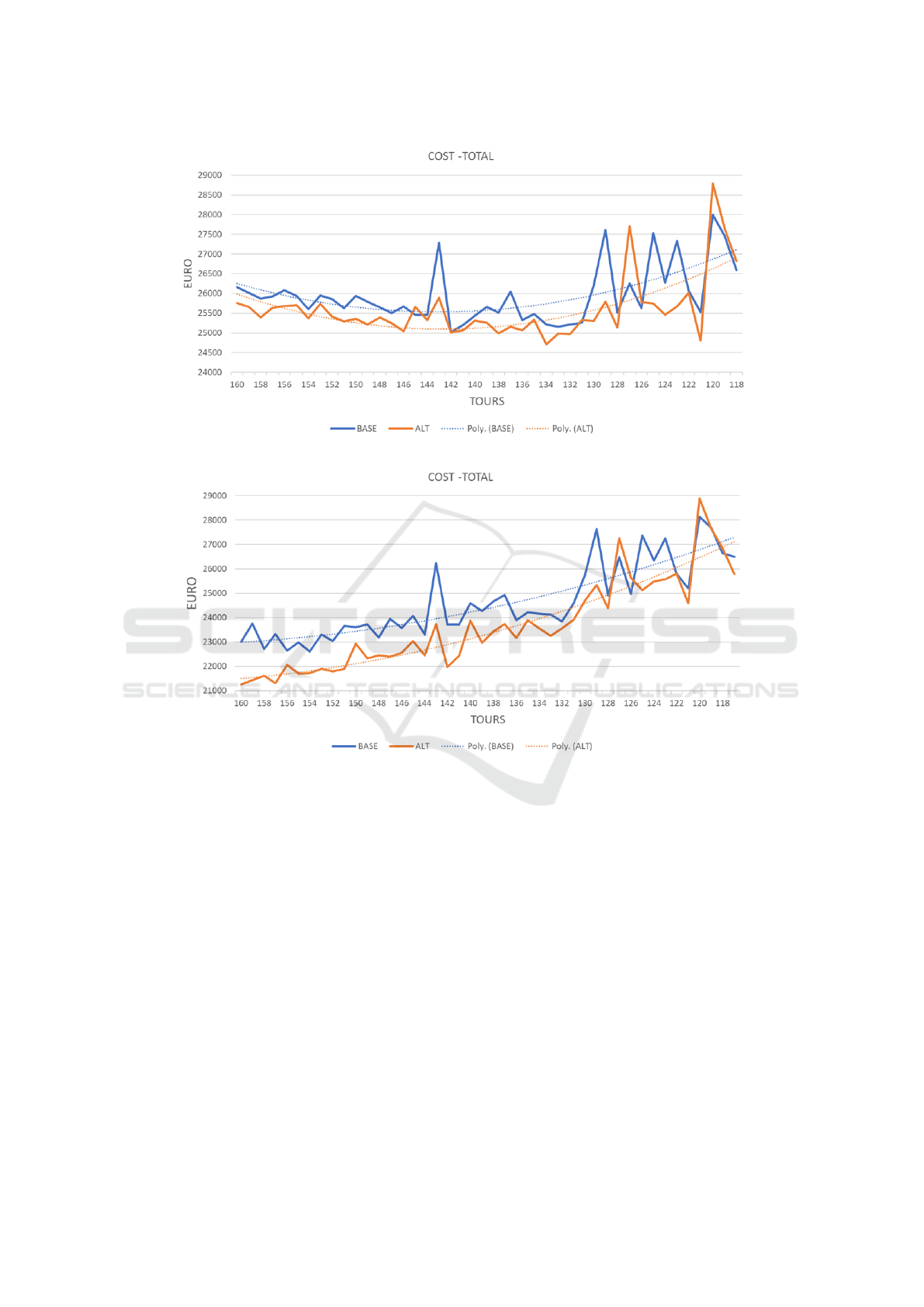
Figure 1: Costs as function of tours, after combining tours.

Figure 2: Costs as function of tours, after integrating tours.

in practice in the distribution centre. Here a smaller

number could be better feasible, what limits the num-

ber needed by the previous point in this list. Also, the

combining of tours leads to a more dynamic demand

on the number of vehicles. In practice vehicles (and

drivers) are contracted some time in advance. A new

process will have to be devised to cope with a more

dynamic usage of vehicles.

ACKNOWLEDGEMENTS

This work has been carried out within the project

‘Self-Organising Logistics in Distribution (SOLiD)’,

supported by NWO (the Netherlands Organisation for

Scientiﬁc Research).

REFERENCES

Baldacci, R., Toth, P., and Vigo, D. (2007). Recent advances

in vehicle routing exact algorithms. 4OR, 5(4):269–

298.

Bertsimas, D. J. and Simchi-Levi, D. (1996). A new

generation of vehicle routing research: robust algo-

rithms, addressing uncertainty. Operations Research,

44(2):286–304.

Bjelde, A., Disser, Y., Hackfeld, J., Hansknecht, C., Lip-

mann, M., Meißner, J., Schewior, K., Schl

oter, M.,

and Stougie, L. (2017). Tight bounds for online tsp

on the line. In Proceedings of the Twenty-Eighth An-

nual ACM-SIAM Symposium on Discrete Algorithms,

pages 994–1005. Society for Industrial and Applied

Mathematics.

Cuda, R., Guastaroba, G., and Speranza, M. G. (2015). A

survey on two-echelon routing problems. Computers

& Operations Research, 55:185–199.

ICORES 2020 - 9th International Conference on Operations Research and Enterprise Systems

334

Jaillet, P. and Wagner, M. R. (2008). Generalized online

routing: New competitive ratios, resource augmenta-

tion, and asymptotic analyses. Operations research,

56(3):745–757.

James, G., Witten, D., Hastie, T., and Tibshirani, R. (2013).

An introduction to statistical learning, volume 112.

Springer.

Ngai, W. K., Kao, B., Chui, C. K., Cheng, R., Chau, M.,

and Yip, K. Y. (2006). Efﬁcient clustering of uncertain

data. In Data Mining, 2006. ICDM’06. Sixth Interna-

tional Conference on, pages 436–445. IEEE.

Phillipson, F. and De Koff, S. (2020). Immediate parcel to

vehicle assignment for cross docking in city logistics:

a dynamic assignment vehicle routing problem. In

Proceedings of 9th International Conference on Op-

erations Research and Enterprise Systems (ICORES).

Pillac, V., Gendreau, M., Gu

eret, C., and Medaglia, A. L.

(2013). A review of dynamic vehicle routing prob-

lems. European Journal of Operational Research,

225(1):1–11.

Ritzinger, U., Puchinger, J., and Hartl, R. F. (2016). A sur-

vey on dynamic and stochastic vehicle routing prob-

lems. International Journal of Production Research,

54(1):215–231.

Savelsbergh, M. and Van Woensel, T. (2016). 50th anniver-

sary invited article—city logistics: Challenges and op-

portunities. Transportation Science, 50(2):579–590.

Tu, D. and Montreuil, B. (2019). Hyper-connected megac-

ity logistics: Multi-tier territory clustering and multi-

plane meshed hub network design. In Proceedings of

IPIC 2019, pages 159–166.

Ulmer, M. W., Brinkmann, J., and Mattfeld, D. C. (2015).

Anticipatory planning for courier, express and parcel

services. In Logistics Management, pages 313–324.

Springer.

Dynamic Assignment Vehicle Routing Problem with Generalised Capacity and Unknown Workload

335