Topological Visualization Method for Understanding the Landscape of

Value Functions and Structure of the State Space in

Reinforcement Learning

Yuki Nakamura

1 a

and Takeshi Shibuya

2 b

1

Graduate School of Systems and Information Engineering, University of Tsukuba, 1-1-1 Tennodai, Tsukuba, Japan

2

Faculty of Engineering, Information and Systems, University of Tsukuba, 1-1-1 Tennodai, Tsukuba, Japan

Keywords:

Reinforcement Learning, Topological Data Analysis, TDA Mapper, Visualization.

Abstract:

Reinforcement learning is a learning framework applied in various ﬁelds in which agents autonomously ac-

quire control rules. Using this method, the designer constructs a state space and reward function and sets

various parameters to obtain ideal performance. The actual performance of the agent depends on the design.

Accordingly, a poor design causes poor performance. In that case, the designer needs to examine the cause of

the poor performance; to do so, it is important for the designer to understand the current agent control rules.

In the case where the state space is less than or equal to two dimensions, visualizing the landscape of the value

function and the structure of the state space is the most powerful method to understand these rules. However,

in other cases, there is no method for such a visualization. In this paper, we propose a method to visualize

the landscape of the value function and the structure of the state space even when the state space has a high

number of dimensions. Concretely, we employ topological data analysis for the visualization. We conﬁrm the

effectiveness of the proposed method via several numerical experiments.

1 INTRODUCTION

Reinforcement learning, in the ﬁeld of machine learn-

ing is a learning framework that autonomously ac-

quires control rules to maximize the rewards from the

environment via the trial and error of agents (Sutton

and Barto, 1998; Matari

´

c, 1997). As a result, it is

possible to lighten the burden on designers of design-

ing complex algorithms (Smart and Pack Kaelbling,

2002).

When acquiring control rules via reinforcement

learning, the designer needs to set up the environment,

learning methods, and parameters; the environment

consists of the state spaces and reward functions, and

the parameters include the learning rates, rates of ex-

ploration and exploitation, and discount rates. Agents

learn by repeated exploration and exploitation under

given circumstances. Therefore, the performance

of the acquired control rules changes depending the

design. If the performance required by the designer

cannot be obtained, it is necessary to investigate the

cause of this failure. Then, the environment, learn-

a

https://orcid.org/0000-0001-9922-890X

b

https://orcid.org/0000-0003-4645-5898

ing method and parameters are reconstructed

and reinforcement learning is performed. By repeat-

ing this cycle, the agent aims to gain the performance

required by the designer. In other words, it is neces-

sary to have a method to investigate causes when the

required performance cannot be obtained.

For such an investigation, it is necessary to under-

stand how the learning is being performed at that time,

that is, it is important to understand the control rules

of the agent. There are several ways to determine this.

Commonly used methods include examining the sum

of rewards acquired for each episode, examining the

control rules of the agent heuristically, and examining

the landscape of the value function and the structure

of the state space. Even though the learning progress

can be understood via a method examining the total

sum of rewards acquired for each episode, it is im-

possible to know why the required performance can-

not be obtained if the rewards cannot be acquired. In

the heuristic method, when the state space is compli-

cated, there are many situations that need to be exam-

ined, which requires a great deal of trials and errors.

In the case where the state space is less than or equal

to two dimensions, visualizing the landscape of the

370

Nakamura, Y. and Shibuya, T.

Topological Visualization Method for Understanding the Landscape of Value Functions and Structure of the State Space in Reinforcement Learning.

DOI: 10.5220/0008913303700377

In Proceedings of the 12th International Conference on Agents and Artiﬁcial Intelligence (ICAART 2020) - Volume 2, pages 370-377

ISBN: 978-989-758-395-7; ISSN: 2184-433X

Copyright

c

value function and the structure of the state space is

the most powerful method to understand the control

rules of the agent. This is because, we can visually

understand the progress of the explore and the evalu-

ation of the state. In this paper, we aim to be able to

understand the control rules of the agent by focusing

on the landscape of the value function and the struc-

ture of the state space. When the state space is low di-

mensional, visualization techniques can represent the

landscape of the value function and the structure of

the state space; however, when the state space is high

dimensional, it becomes difﬁcult to visualize.

Therefore, the purpose of this study is to visualize

the landscape of the value function and the structure

of the state space when the state space is high dimen-

sional. Additionally, we show that this visualization is

useful for understanding the control rules of the agent

in reinforcement learning.

2 BACKGROUND

Reinforcement learning involves learning motion se-

lection for a certain state to maximize the reward (Sut-

ton and Barto, 1998). Many algorithms for reinforce-

ment learning are based on estimating value func-

tions. These function are classiﬁed into two types:

state value functions and action value functions. A

state value function is represented by V (s) and eval-

uates how much value an agent has in a given state.

An action value function is represented by Q(s, a) and

evaluates how much value is gained by performing a

given action in a given state for an agent.

2.1 Q-learning

Q-learning (Watkins and Dayan, 1992) is a value-

updating algorithm in reinforcement learning that up-

dates the action value function Q(s

t

, a

t

) using Equa-

tion (1).

Q(s

t

, a

t

) ← (1 −α)Q(s

t

, a

t

) + α

h

r

t+1

+ γ max

a

Q(s

t+1

, a)

i

(1)

Here, α is a parameter called the step-size, where 0 ≤

α ≤ 1. This parameter controls the rate at which the

action value function Q(s

t

, a

t

) is updated.

The ε-greedy method is often used as a behavioral

selection method in Q-learning, where 0 ≤ ε ≤ 1. This

is a method of taking random action with a probability

of ε and taking the action probability function with the

largest action with the probability of 1 − ε. In other

words, the larger the value of ε, the higher the explo-

ration rate, and the smaller the value of ε, the higher

the exploitation rate.

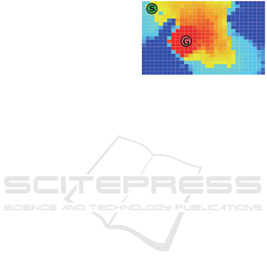
Figure 1: A heat map of learning how to climb a virtual

volcano from S (the start) to G (the goal) at the summit.

2.2 Heat Map

A heat map can be used as a method to visualize the

landscape of the value function and the structure of

the state space; an example of heat map is shown in

Figure 1. Here, a two-dimensional state space is de-

ﬁned in the domain and the state value function is rep-

resented by the color shading. The heat map in Fig-

ure 1 represents a learning of how to climb a virtual

volcano from S (the start) to G (the goal) at the sum-

mit. In general, an agent has a policy to perform a

state transition to a state higher than the state value

of the existing state. In other words, when visual-

ized with this heat map, the transition to a warmer

color state is taken to be the policy and the probabil-

ity of repeating the state transition to a warmer color

state where a transition is possible is high. By analyz-

ing the heat map, the designer can roughly understand

how the agent repeats the state transition. Therefore,

the heat map visualizes the structure of the state space

and the landscape of the value function and is useful

for understanding the agent control rule.

However, it is rare for a heat map to be able to

visualize the structure the of state space and the land-

scape of the value function. This is because a heat

map has only two dimensions in the state space and it

is difﬁcult to use it in the case of three or more dimen-

sions. Moreover, in the example of the virtual volcano

in Figure 1, it is assumed that the state transition can

be performed in the adjacent state; however, in actual-

ity, the state transition cannot be performed in the ad-

jacent state nor can the state transition be performed

in the non-adjacent state. If a system that can visual-

ize the structure of the state space and the landscape

of the value function exists, even if such a state space

has high dimensions or the structure of the state space

is complex, it would be useful. This is the purpose of

this study.

Topological Visualization Method for Understanding the Landscape of Value Functions and Structure of the State Space in Reinforcement

Learning

371

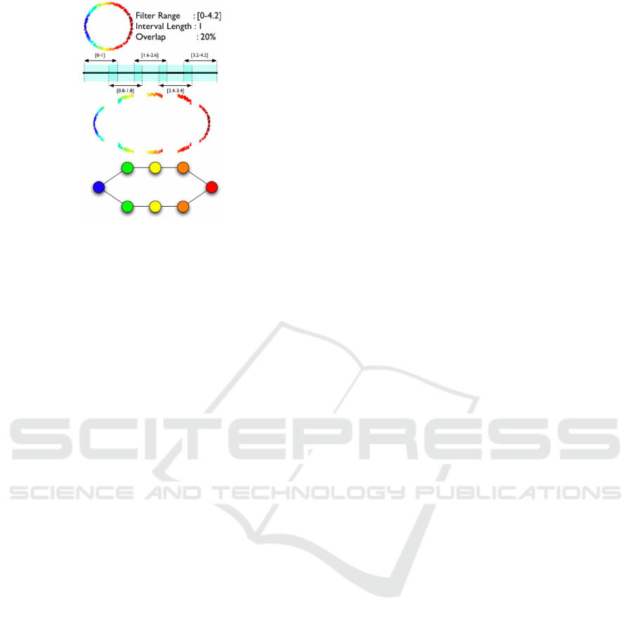
Figure 2: The TDA Mapper (from Singh et al. (Singh et al.,

2007) Figure 1).

2.3 TDA Mapper

In recent years, the TDA Mapper has attracted atten-

tion as a method for analyzing high dimensional and

large-scale data and as a big data analysis technol-

ogy that makes it easier for users to understand data

(Singh et al., 2007; Hamada and Chiba, 2017; Wang

et al., 2015). This is a method to topologically ana-

lyze data and create a graph with a topological struc-

ture similar to the original data. TDA Mapper mainly

analyzes point clouds, and uses the distance matrix of

point clouds as input data. The topological analysis

of high dimensional data is the focus of this study.

Figure 2 shows how to create a graph using TDA

Mapper. This is an example of creating a graph with

circularly distributed data while maintaining the topo-

logical structure. The graph creation algorithm in par-

ticular is shown. We analyze a point cloud

X =



x

1

, . . . , x

n



.

The point cloud X is distributed in a circle.

1. By deﬁning the ﬁlter function,

h : X → R,

on the point cloud X, a ﬁlter value h(x) is given to

each point x. The circle is given a ﬁlter value that

increases from left to right.

2. The range h(X ) of the ﬁlter function is covered

with m intervals, I

1

, . . . , I

m

, and the point group X

is divided into level sets:

X

i

=



x ∈ X | h(x) ∈ I

i



.

Here, the lengths of the divided intervals are all

equal and the adjacent intervals I

i

and I

i+1

both

overlap by p% of the interval length. The example

in the Figure 2 is divided into ﬁve intervals with

20% overlap.

3. Each level set X

i

is clustered using an arbitrary

method and divided into clusters:

X

i

=

M

j

X

j

i

,

where

L

stands for direct sum and is synonymous

with

X

i

=

[

j

X

j

i

, X

j

i

\

X

j

0

i

= φ ( j 6= j

0

).

The adjacency relationships of the clusters X

j

i

are

expressed as a graph. Speciﬁcally, with a cluster

as a vertex, a graph

G

h

(X) =

(

V =



X

j

i



E =



(X

j

i

, X

k

i+1

) | X

j

i

T

X

k

i+1

6= φ



is constructed in which the edges are extended be-

tween the overlapping clusters belonging to adja-

cent levels. In Figure 2, the vertices of the graph

are ordered according to the level.

TDA Mapper requires the user to set many pa-

rameters at the time of graph creation; These param-

eters are the number of divisions of the ﬁlter function

range, the overlap ratio, and the clustering method.

From this, depending on the settings of the parame-

ters, the shape of the graph can differ greatly and it

is difﬁcult to determine whether the output graph is

useful. The proposed method aims to improve this

problem as well.

3 THE PROPOSED METHOD: RL

MAPPER

We propose a method to visualize the structure of the

state space and the landscape of the value function

even when the state space is high dimensional and

complex. The proposed method is named RL Mapper,

where RL is an abbreviation for reinforcement lean-

ing. In this method, we modiﬁed the 2.3 TDA Mapper

algorithm to be appropriate for reinforcement learn-

ing. TDA Mapper analyzes point clouds and uses data

on the distance between points. On the other hand, RL

Mapper analyzes the landscape of the value function

and the structure of the state space. We make it possi-

ble to represent the landscape of the value function by

using state value data. Additionally, we make it possi-

ble to deﬁne the distance between states by using the

history of agent state transitions.

Here, we describe the speciﬁc algorithm. We visu-

alize the landscape of the value function and the struc-

ture of the state space of the state set,

S =



s

1

, . . . , s

n



,

which is completely learned or under learning.

ICAART 2020 - 12th International Conference on Agents and Artiﬁcial Intelligence

372

1. We deﬁne the ﬁlter function as the state value

function

v : S → R.

We give a ﬁlter value v(s) for each state s ∈ S.

2. We deﬁne m uncovering intervals I

1

, . . . , I

m

in the

range v(s) of the ﬁlter function. We divide the

state set S into level sets:

S

i

=



s ∈ S | v(s) ∈ I

i



.

Here, the sizes of the sections I

1

, . . . , I

m

are equal.

3. We cluster each level set S

i

and divide it into clus-

ters:

S

i

=

M

j

S

j

i

.

Here, we describe the clustering method used in

this approach. We deﬁne a set of states having a

history of state transitions between the states s ∈

S

i

of the level set S

i

as one cluster. We construct a

graph

G

v

(S) =











V =



S

j

i



E =



(S

j

i

, S

l

k

) | S

j

i

and S

l

k

have one

or more pairs of state pairs S

j

i

and S

l

k

that can transition between states



with nodes as clusters and edges deﬁned below.

We call this graph, G

v

(S), the topological state

graph. We show an example of a topological state

graph in Figure 3.

The features of the topological state graph are as

follows.

• A node is a set of “state value close” and “state

transitionable” states.

• The color density of a node is the average of the

state value of the state clustered on that node.

– A warm color indicates a high state value.

– A cool color indicates a low state value.

• We give the node a number x-y.

– x is a number indicating the interval of the state

value, where the state value is larger if the num-

ber is larger.

– y is the cluster label within the x interval.

• The size of a node is correlated to the number of

states included in that node.

• Between nodes connected by an edge, there are

one or more state pairs capable of a state transi-

tion.

1·1

1·2

1·3

1·4

2·1

2·2

2·3

3·1

3·2

4·1

4·2

5·1

5·2

6·1

6·2

7·1

7·2

8·1

8·2

9·1

10·1

node num qvalue

10·1 9 96.1

9·1 17 85.59

8·2 9 75.91

8·1 9 75.91

7·2 10 66.37

7·1 12 65.83

6·2 8 57.33

6·1 12 55.92

5·2 17 45.84

5·1 24 45.64

4·2 21 35.41

4·1 18 35.74

3·2 90 25.39

3·1 29 25.77

2·3 36 16.86

2·2 54 15.27

2·1 48 15.42

1·4 1 1

1·3 1 1

1·2 15 10.37

1·1 1 1

Figure 3: Topological stage graph.

The inputs to RL Mapper are state values of each state

and adjacency matrix representing the history of state

transitions based on agent experience. The only pa-

rameter set by the user is the number of divisions of

the ﬁlter value for the state value function. In rein-

forcement learning, it is difﬁcult to deﬁne the dis-

tance between states; therefore, we performed clus-

tering using the history of the state transitions. This

makes it possible to store the structure of the state

space with higher accuracy. Moreover, because the

number of parameters is small, it is easy for the de-

signer to understand how the graph visually changes

owing to adjustments to the parameters.

4 EXPERIMENTS

The topological state graph, which visualizes the

landscape of the value function and the structure of

the state space with RL Mapper, is shown via experi-

ments to be useful for understanding the agent con-

trol rules. We experimented in two situations. In

Experiment 1, the state space is a two-dimensional

path search problem, and in Experiment 2 the state

space is a four-dimensional taxi task. In Experiment

1, by comparing the heat map with the topological

state graph, we show that the topological state graph

reproduces the utility of the heat map. We divided Ex-

periment 1 into 1-A and 1-B in which only the value

of reward was changed. In this way, we show that

by visualizing the landscape of the value function and

the structure of the state space, it is possible for the

designer to understand the difference in the control

Topological Visualization Method for Understanding the Landscape of Value Functions and Structure of the State Space in Reinforcement

Learning

373

rules of the agent caused by the change of the reward

function. In Experiment 2, we show that RL Map-

per is useful in the case of the high dimensional state

space as well as in the low dimensional one.

4.1 Two-dimensional Path Search

Problem

4.1.1 Outline of the Experiment

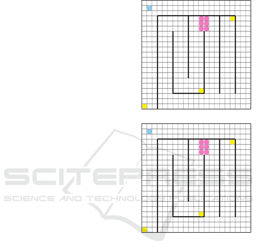
We divided the two-dimensional path search prob-

lem into Experiment 1-A and 1-B. Figure 4 shows

the environment of the route search problem used in

Experiment 1-A, and Figure 5 shows the same for

Experiment 1-B. In both experiments, 1-A and 1-B,

the agent is on a two-dimensional plane that satis-

ﬁes x, y ∈ Z, 0 ≤ x, y ≤ 21. The state space is two-

dimensional consisting of the x coordinates and y co-

ordinates. The agent can recognize only the current

coordinates and the obtained reward and cannot rec-

ognize other environmental information.

The agent, as an action can move one square in

the vertical or horizontal direction. The agent cannot

move while in the state partitioned by the wall (the

thick line) and remains in the original state when se-

lecting an action to move toward the wall. Experiment

1-A starts at S, and when the agent reaches a point in-

dicated as 30, 50, 1000, or -500, we reward the agent

with 30, 50, 1000, or -500, respectively. Addition-

ally, when the agent reaches a point indicated as 30,

50, or 1000, the episode ends and the next episode

starts from the point of S. Similarly, if Experiment

1-B starts at S, and the agent reaches the points in-

dicated as 30, 50, 100, or -40, we reward the agent

with 30, 50, 100, or -40, respectively. When the agent

reaches a point indicated as 30, 50, or 100, the episode

ends and the next episode starts from the point S.

We use Q-learning and the set step-size α = 0.5,

explore ratio ε = 0.999

n

, where n is the number of

episodes and the discount rate γ = 0.95. The number

of divisions in the range of the ﬁlter function, which

is a parameter of the RL Mapper, is 10.

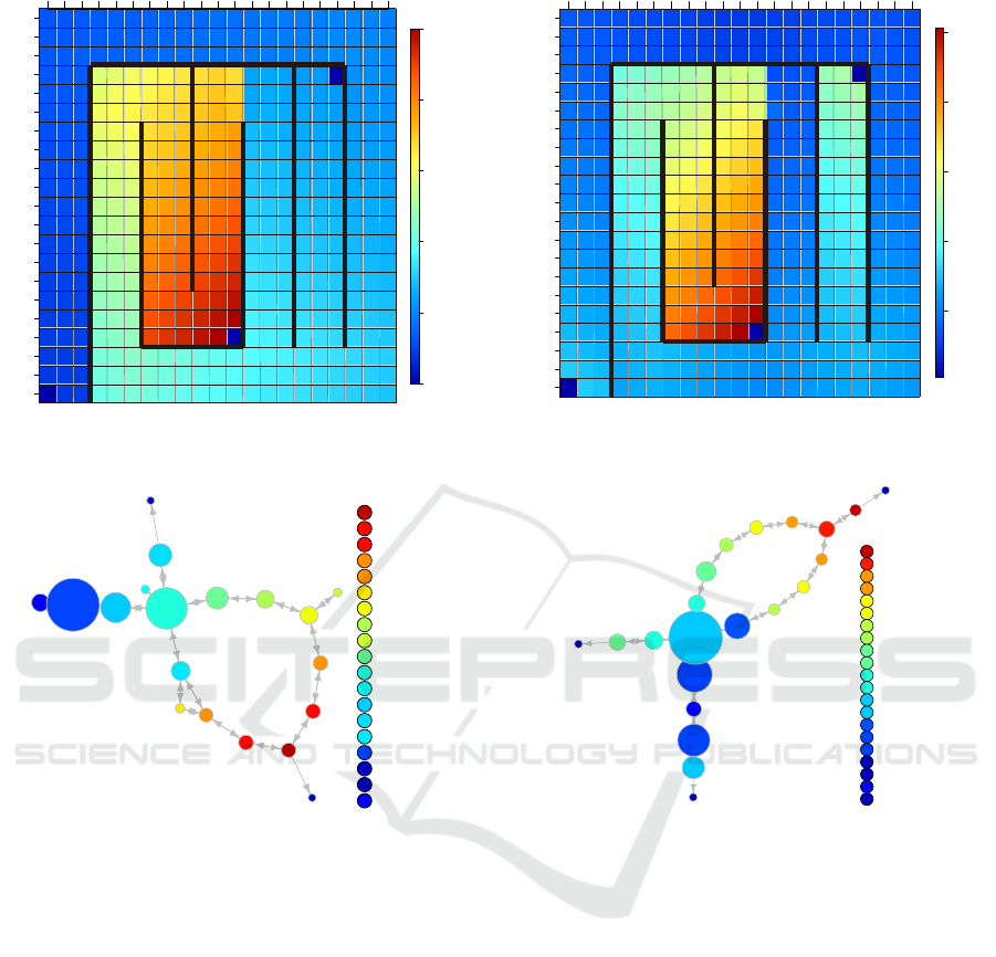
4.1.2 Results and Discussion

We show the heat map and state phase graph of 10,000

episodes in Experiment 1-A in Figures 6 and 7, re-

spectively. The labels of the nodes correspond to the

labels of the heat map.

The graphs of the 10,000 episodes shown in Fig-

ures 6 and 7 are for after the learning has been com-

pleted. The agent has a policy of repeating state tran-

sitions to higher states of the state value function.

Therefore, we can see from the heat map in Figure

Figure 4: Environment of Experiment 1-A.

Figure 5: Environment of Experiment 1-B.

6 that the agent has a state transition from 2-1 to 3-

3 to 4-1 to 5-1 to 6-2 to 7-1 to 8-1 to 9-1 to 10-1 to

1-2 as the control rule. As an exception, in 1-2, the

state value remains low because the agent receives a

reward and the episode ends. That is, the agent aims

to reach the state where it can earn a reward of 1000.

Here, there is one other way to reach the state where

the agent can earn a reward of 1000. It is a path where

the agent transitions from 2-1 to 3-3 to 4-1 to 3-1 to

7-2 or 8-2 to 9-2 to 10-1 to 1-2. However, the agent

does not have this route as the control rule because the

state value decreases at the state transition from 4-1 to

3-1. Similarly, we can see from the topological state

graph in Figure 7 that the agent has a state transition

from 2-1 to 3-3 to 4-1 to 5-1 to 6-2 to 7-1 to 8-1 to

9-1 to 10-1 to 1-2 as the control rule. The topological

state graph also shows another way to reach the state

ICAART 2020 - 12th International Conference on Agents and Artiﬁcial Intelligence

374

0

200

400

600

800

1000

1 2 3 4567 8 9 10 11 12 13 14 15 16 17 18 19 20 21

21

20

19

18

17

16

15

14

13

12

11

10

9

8

7

6

5

4

3

2

1

1·1

1·2

1·3

2·1

2·1 2·1

2·1

2·

1

2·1

3·1

3·2

3·3

3·4

4·1

4·

1

4·1

5·1

6·1

6·2

7·1

7·2

7·2 7·2

7·2

8·1

8·2

8

·2

8·2

9·1

9·2

10·1

Figure 6: Heat map for 10,000 episodes in Experi-

ment 1-A.

1·1

1·2

1·3

2·1

3·1

3·2

3·3

3·4

4·1

5·1

6·1

6·2

7·1

7·2

8·1

8·2

9·1

9·2

10·1

node num qvalue

10·1 14 953.6

9·2 15 855.2

9·1 15 855.2

8·2 13 751.3

8·1 15 749.7

7·2 5 685

7·1 21 643.5

6·2 21 546.9

6·1 3 585.9

5·1 30 444.3

4·1 69 337.4

3·4 3 295.4

3·3 46 248.4

3·2 32 263.1

3·1 24 270.3

2·1 92 147.3

1·3 1 1

1·2 1 1

1·1 21 87.22

Figure 7: Topological state graph for 10,000 episodes

in Experiment 1-A.

where the agent can earn a reward of 1000. we can

see that the agent does not have this route as the con-

trol rule because the state value decreases at the state

transition from 4-1 to 3-1.

Next, we show the heat map and state phase graph

of the 10,000 episodes in Experiment 1-B in Figures 8

and 9, respectively. The graphs of the 10,000 episodes

shown in Figure 8 and 9 are for after the learning has

been completed. We can see from the heat map in

Figure 8 that the agent has a state transition from 2-1

to 3-1 to 1-1 as the control rule. That is, the agent aims

to reach the state where it can earn a reward of 30. The

agent does not aim to reach a state where it can earn

rewards of 50 or 100. This is because this path has a

reduced state value at the state transition from 2-1 to

1-2. Similarly, we can see from the topological state

graph in Figure 9 that the agent has a state transition

from 2-1 to 3-1 to 1-1 as the control rule.

From Experiments 1-A and 1-B, we can see that

20

40

60

80

100

123456789 10 11 12 13 14 15 16 17 18 19 20 21

21

20

19

18

17

16

15

14

13

12

11

10

9

8

7

6

5

4

3

2

1

1·1

1·2 1·2

1·2

1·3

1·4

2·1

2·1 2·1 2·2

2·2

2·3

2

·3

2·3

3·1

3·2

3·

2

3·2

4·1

4·2

5·1

2·51·5

5·2

6·1

6·2

7·1

7·2

8·1

8·2

9·1

10·1

Figure 8: Heat map for 10,000 episodes in Experi-

ment 1-B.

1·1

1·2

1·3

1·4

2·1

2·2

2·3

3·1

3·2

4·1

4·2

5·1

5·2

6·1

6·2

7·1

7·2

8·1

8·2

9·1

10·1

node num qvalue

10·1 9 96.1

9·1 17 85.59

8·2 9 75.91

8·1 9 75.91

7·2 10 66.37

7·1 12 65.83

6·2 8 57.33

6·1 12 55.92

5·2 17 45.84

5·1 24 45.64

4·2 21 35.41

4·1 18 35.74

3·2 90 25.39

3·1 29 25.77

2·3 36 16.86

2·2 54 15.27

2·1 48 15.42

1·4 1 1

1·3 1 1

1·2 15 10.37

1·1 1 1

Figure 9: Topological state graph for 10,000 episodes

in Experiment 1-B.

the topological state graph output by RL Mapper pre-

serves the landscape of the value function and the

structure of the state space. Additionally, we ﬁnd

that the agent control rules are different when com-

paring Experiments 1-A and 1-B. The difference in

the control rules results from the difference in the de-

sign of the reward function. The designer can visually

understand the differences in control rules using the

topological state graph. Therefore, topological state

graphs are useful for understanding the control rules

of agents.

Topological Visualization Method for Understanding the Landscape of Value Functions and Structure of the State Space in Reinforcement

Learning

375

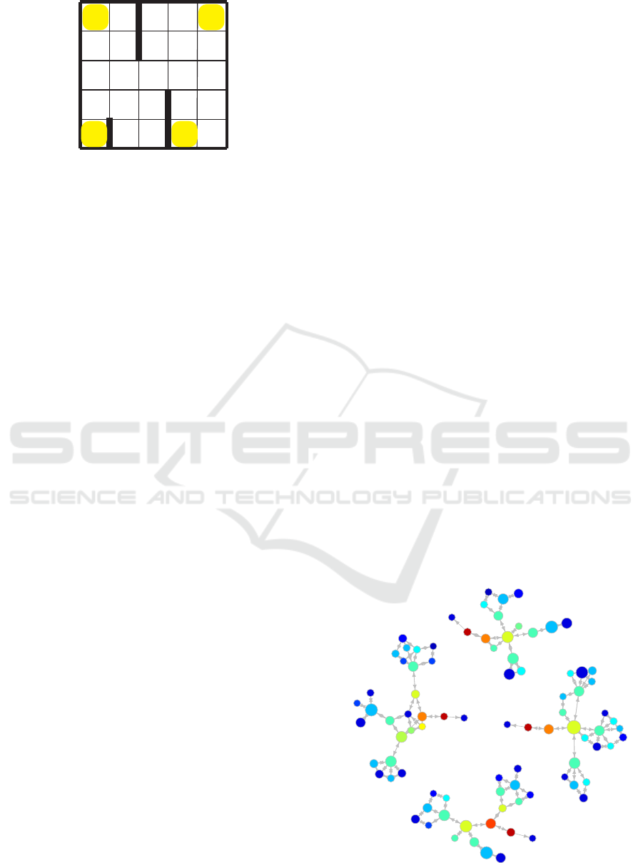
Figure 10: The taxi task.

4.2 Four-dimensional Taxi Task

4.2.1 Outline of the Experiment

The taxi task is to pick up a passenger in the environ-

ment shown in Figure 10 and carry them to the desti-

nation (S¸ ims¸ek et al., 2005). The agent here is a taxi.

A taxi, a passenger are located on a two-dimensional

plane that satisﬁes x, y ∈ Z, 0 ≤ x, y ≤ 5. The loca-

tions and destinations of the passengers are randomly

selected from the locations indicated by A, B, C, and

D. The initial position of the taxi is randomly selected

from the positions satisfying the above equation. At

each location, taxis have one choice of action: move

one square north, south, east, or west, pick up a pas-

senger, or drop off a passenger. The action of picking

up a passenger is only possible if the passenger is in

the same position as the taxi. Similarly, dropping off

a passenger is only possible if the passenger is in the

taxi and the taxi is at the destination. additionally,

agents cannot transition between pairs of states sep-

arated by walls (the thick line). If the agent chooses

to move toward a wall, it remains in its original state.

We reward the agent with 20 if the agent can deliver

the passenger to the destination. Additionally, when

we reward an agent, we end that episode and move to

the next episode. The state space is four-dimensional

consisting of the x coordinates, y coordinates, passen-

ger status, and destination location.

We use Q-learning and the set step-size α = 0.5,

the explore ratio ε = 0.3, and the discount rate γ =

0.9. The number of divisions in the range of the ﬁlter

function, which is a parameter of the RL Mapper, is

6.

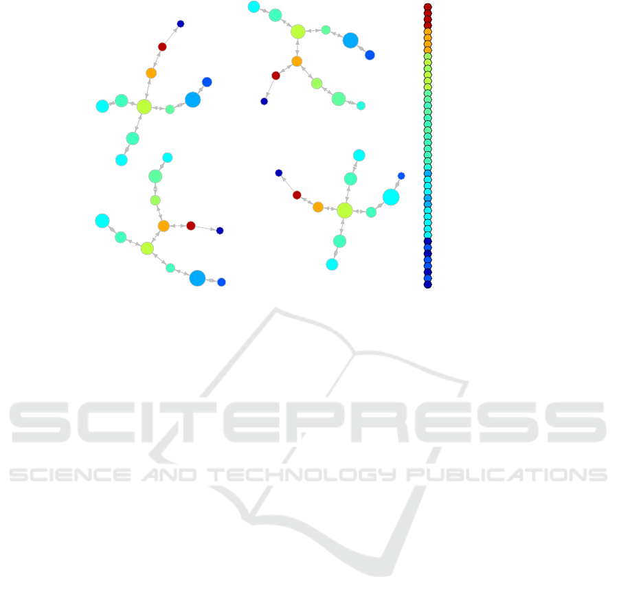
4.2.2 Results and Discussion

We show the state phase graph for 5000 and 10,000

episodes in the Figure 11 and 12. RL Mapper can

also be used on the data during learning. The 5000

episodes are for the data during the learning, and the

10,000 episodes are for the data after the learning. We

compared the topological state graphs for the 5000

episodes in Figure 11 to the 10,000 episodes in Figure

12. We can see that the topological state graph for the

10,000 episodes has fewer nodes and edges and that

the graph is simpler than that for 5000 episodes. This

is because the learning process has smoothened the

landscape of the values. Additionally, we can see that

the graph is composed of four groups in the topolog-

ical state graphs for 5000 and 10,000 episodes. This

is because there are four destinations, which are sep-

arate tasks, and there is no state transition between

tasks.

Considering the topological state graph for 10,000

episodes in the Figure 12, we ﬁnd that there are three

routes going to the high-value nodes 6-1, 6-2, 6-3,

and 6-4, and that these routes join to reach high-value

nodes. This is due to the three locations of the pas-

sengers not boarding at each destination. When a pas-

senger takes a taxi, they transition to high-value nodes

and reach nodes 1-1, 1-3, 1-6 and 1-8, where rewards

can be obtained.

Therefore, in the case of high dimensional state

space, RL Mapper can visualize the landscape of the

value function and the structure of the state space.

Moreover, we were able to understand the rough con-

trol rule of the agent using the topological state graph.

5 CONCLUSIONS

The purpose of this paper is to allow the designer to

understand the agent control rules by visualizing the

landscape of the value function and the structure of

the state space when the state space is high dimen-

1·1

1·2

1·

3

1·4

1·5

1·6

1·7

1·8

1·9

1·10

1·11

1·12

1·13

1·14

1·15

1·16

1·17

1·18

1·19

1·20

1·21

1·22

1·23

1·24

1·25

1·26

1·27

1·28

1·29

2·1

2·2

2·3

2·4

2·5

2·6

2·7

2·8

2·9

2·10

2·11

2·12

2·13

2·14

2·15

2·16

2·17

2·18

2·19

2·20

2·21

2·22

2·23

2·24

2·25

2·26

3·1

3·2

3·3

3·4

3·5

3·6

3·7

3·8

3·9

3·10

3·11

3·12

3·13

3·14

3·15

3·16

3·17

3·18

4·1

4·2

4·3

4·4

4·5

4·6

4·7

5·1

5·2

5·3

5·4

6·1

6·2

6·3

6·4

Figure 11: Topological state graph for 5000 episodes.

ICAART 2020 - 12th International Conference on Agents and Artiﬁcial Intelligence

376

1·1

1·2

1·3

1·4

1·5

1·6

1·7

1·8

2·1

2·2

2·3

2·4

2·5

2·6

2·7

2·8

2·9

2·10

2·11

2·12

3·1

3·2

3·3

3·4

3·5

3·6

3·7

3·8

3·9

3·10

3·11

3·12

4·1

4·2

4·3

4·4

4·5

4·6

5·1

5·2

5·3

5·4

6·1

6·2

6·3

6·4

node num qvalue

6·4 3 19.51

6·3 4 19.33

6·2 3 19.51

6·1 3 19.51

5·4 7 15.96

5·3 9 15.99

5·2 7 15.96

5·1 7 15.96

4·6 8 11.9

4·5 15 12.39

4·4 6 11.95

4·3 12 12.6

4·2 16 12.31

4·1 18 12.24

3·12 14 9.097

3·11 4 9.272

3·10 12 8.872

3·9 13 9.028

3·8 9 8.819

3·7 4 8.797

3·6 4 9.272

3·5 12 8.872

3·4 12 8.872

3·3 12 8.872

3·2 7 8.897

3·1 12 8.872

2·12 3 7.044

2·11 18 5.753

2·10 10 6.594

2·9 6 6.814

2·8 15 6.386

2·7 19 5.958

2·6 18 5.753

2·5 12 6.649

2·4 10 6.594

2·3 10 6.594

2·2 20 6.113

2·1 10 6.594

1·8 1 1

1·7 6 4.023

1·6 1 1

1·5 3 4.16

1·4 6 4.023

1·3 1 1

1·2 1 4.303

1·1 1 1

Figure 12: Topological state graph for 10,000 episodes.

sional. When the state space is low dimensional, a

method of visualizing the landscape of the value func-

tion and the structure of the state space already ex-

ists, the heat map; however, when the state space is

high dimensional, there is no method for such a vi-

sualization. Therefore, we proposed RL Mapper, a

visualization method that focuses on the topological

structure of the data. We examined the correspon-

dence between a heat map and a topological state

graph when the state space was two dimensional using

a path search problem and showed that the topologi-

cal state graph retains the usefulness of a heat map.

We also showed that the visualization of the value

function landscape and the state space structure in RL

Mapper is useful for understanding the agent control

rules. Additionally, using the taxi task, we showed

that RL Mapper can provide the same visualization

even when the state space is four dimensional. There-

fore, RL Mapper can visualize the landscape of the

value function and the structure of the state space in

the case of a high dimensional state space. We also

demonstrated that this visualization is useful for un-

derstanding the control rules of agents.

REFERENCES

S¸ ims¸ek, O., Wolfe, A. P., and Barto, A. G. (2005). Identify-

ing useful subgoals in reinforcement learning by local

graph partitioning. In Proceedings of the 22Nd In-

ternational Conference on Machine Learning, ICML

’05, pages 816–823, New York, NY, USA. ACM.

Hamada, N. and Chiba, K. (2017). Knee point analysis

of many-objective pareto fronts based on reeb graph.

In 2017 IEEE Congress on Evolutionary Computation

(CEC), pages 1603–1612.

Matari

´

c, M. J. (1997). Reinforcement learning in the multi-

robot domain. Auton. Robots, 4(1):73–83.

Singh, G., Memoli, F., and Carlsson, G. (2007). Topolog-

ical Methods for the Analysis of High Dimensional

Data Sets and 3D Object Recognition. In Botsch, M.,

Pajarola, R., Chen, B., and Zwicker, M., editors, Eu-

rographics Symposium on Point-Based Graphics. The

Eurographics Association.

Smart, W. D. and Pack Kaelbling, L. (2002). Effective rein-

forcement learning for mobile robots. In Proceedings

2002 IEEE International Conference on Robotics and

Automation (Cat. No.02CH37292), volume 4, pages

3404–3410 vol.4.

Sutton, R. S. and Barto, A. G. (1998). Introduction to Re-

inforcement Learning. MIT Press, Cambridge, MA,

USA, 1st edition.

Wang, L., Wang, G., and Alexander, C. A. (2015). Big data

and visualization: Methods, challenges and technol-

ogy progress. Digital Technologies, 1(1):33–38.

Watkins, C. J. C. H. and Dayan, P. (1992). Technical note:

q-learning. Mach. Learn., 8(3-4):279–292.

Topological Visualization Method for Understanding the Landscape of Value Functions and Structure of the State Space in Reinforcement

Learning

377