Ultrasound Imaging: Beamforming Techniques

Soufiane Dangoury

, Mohammed Sadik

, Abdelhakim Alali

and Saad Abouzahir

High School of Electrical and Mechanical Engineering (ENSEM) - Hassan II University of Casablanca, Morocco

Ben M’Sik faculty of Science - Hassan II University of Casablanca, Morocco

Keywords: Ultrasound imaging, Spatial resolution, Beamforming, DAS, DMAS, MV.

Abstract: Ultrasound medical imaging continues to progress and allows practitioners to have a fundamental tool to make

a good diagnosis and be able to take the best decisions for different medical fields and contributes to the

improvement of the medical examination of different diseases. Researchers continue to develop approaches

to improve the quality of the ultrasound image. Images generated by the ultrasound system requires high

spatial resolutions for a better detection of the organs boundaries. However, images generated by the system

suffers from artefacts (e.g. side lobs, grate lobs. etc) which negatively impact the quality of the ultrasound

image. Several approaches have been proposed to enhance the spatial resolutions; however, their

performances differ depending on the degree of artefacts. In this paper we present three methods of

beamforming which has a serious role in the process of US image generation. The first one concern delay-

and-sum (DAS) algorithm which is the most commonly used as beamformer , the second is an extension of

DAS (DMAS: Delay Multiply and Sum) and the last one is MVB ( Minimum Variance Beamforming) technic.

the results show the difference between the three beamforming methods. We try in this work to identify

thehiglights and limits of each of these methods.

1 INTRODUCTION

Ultrasound medical imaging is an imaging technique

for exploring the inner structures of the human body.

Up to date, several sophisticated imaging techniques

has been developed to provide better quality images.

Indeed, ultrasound is still used due to its simplicity

and safety for practitioners and patients as it does not

rely on ionizing radiation and has no negative impact

on vital organs. However, the drawbacks of the

ultrasound imaging reside in the quality of the signal

which suffer from artefacts, and its accuracy depends

on the skills of the practitioner. Several works have

been carried out to improve the quality of the

ultrasound image.

The delay and sum (DAS) technic is a part of non-

adaptive beamformer, it improves the resolution

easily around the focal point but with a greater depth,

the method becomes ineffective, because of off-axis

interference (Hoskins, 2010).

Authors in (Holfort, Gran & Jensen, 2009)

https://orcid.org/0000-0000-0000-0000

propose an adaptive beamformer technic to overcome

the depth issues as the minimum variance

beamforming (MVB); their approach relies on the

reduction of the interference, but it has also its limits,

the SNR of the received signals decrease.

Authors in (Haji and al, 2018) take advantage of

the promising results of MV for harmonic imaging.

The authors in (Nguyen and Prager, 2016) show

that bidirectional pixel-based focusing (BiPBF) leads

to improve the SNR of the image signals especially in

the regions far from the focal points; this improves

the contrast of the

images.

Authors in (Asl and Deylami, 2018), propose a

method based

on dominant mode rejection (DMR),

that approximate the covariance matrix using only

some of the largest dominant modes in the dominant

subspace; this method does not need a full matrix

inversion which reduces the computation realized in

normal case of the minimum variance beamforming

(MVB) but with closed results. In (Matrone, and al,

2015) propose a non-adaptive method which slightly

similar to DAS, the Delay-Multiply-And-Sum

(DMAS) provides an interest point spread function

than DAS.

Our contribution in this paper consists of a

comparing of three mostly used methods in US

imaging (DAS, DMAS and MV) and show their

advantage and limits. We use, in this study, some

metrics like FWHM end PSL to evaluate these

methods graphically.

This paper is organized as follows: In section II,

we explain the basic concept of beamforming by

focusing on the DAS method. Section III will be

dedicated to the presentation of the DMAS method.

In section IV, a description of the Minimum Variance

beamforming (MVB) method is given. The section V,

will focus on a discussion of the three methods and

their strengths and weaknesses and limits. And in last

section, we conclude by dressing some issues for next

exploration explore.

2 THE BASIC ASPECTS OF

ULTRASOUND BEAMS

First, the lateral resolution is high when the width of

the beam of ultrasound is narrow (Asl and Deylami,

2018).

So, there is a trade-off between the lateral

resolution and the width of the beam. The shape of

the ultrasound beam is important for detecting more

details along all the image depths, but unfortunately,

it is difficult to control easily the beams’ shape

because the diverges rapidly after being transmit

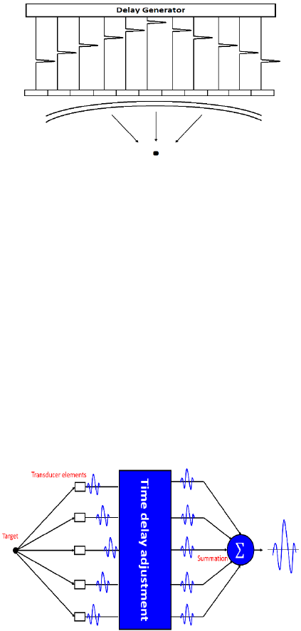
2.1 Focusing

This technique makes it possible to focus the beam on

one point at a given scan line chosen by the operator

and making the beam very narrow and concentrate

more power on the corresponding points, this is more

likely to increase the lateral resolution considerably

in the chosen region. However, this negatively impact

the frame rate as it is computationally intensive. This

issue can be resolved by shifting the active group of

elements by cancelling one element from one side end

and enabling a new one to the other.

Figure 1: Beam technic principle.

As we can see in Figure 1, all the transmitted

pulses from the active aperture must arrive

simultaneously at one point. This is achieved by

controlling the excitation delay between different

element.

According to (Hoskins, 2010) Among the most

used beamforming methods in commercialized

ultrasound the delay and sum (DAS) beamformer due

the simplicity it presents when setting up which is

simply based on obtaining the radio frequency signal

from different channel by summing them after

applying an appropriate delay.

2.2 Delay and Sum Beamforming

Method

Figure 2: Simplified schematic of DAS.

When we are receiving echo signals from a point

all the receives signals form the active aperture must

be summed together to produce the final signal to the

considered scan line in this same time and we can

achieve that by controlling delay between different

element consist the aperture.

DAS technic beamformer is easy to apply and

robust in noisy environments, meanwhile, it performs

well in real-time ultrasound imaging (Hoskins, 2010).

Although, the resulting signal suffers from trade-off

between the main lobe level and the side lobe width

(Haji and al, 2018). Improving the image quality of

ultrasound system has become the focus of many

researchers in this field (Mohades and al, 2018).

The DAS-beamformed formula is obtained as:

𝑦



𝑡   𝑆



t  ∆𝑡









(1)

Where y

DAS

is the received signal at the j’th scan;

N is the number of active elements, and Δtj is the

delay time applied to the received signal of the j’th

scan (Jongin and al, 2016).

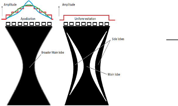
2.3 Apodization

Apodization is a process of beam forming, it can be

used in both transmit and receive beamforming. This

process consists of giving different weightings to

transmit or received signals from different elements

constituting the active part of the probe (aperture). In

transmitting, an element is excited more than other,

and in receiving one signal is more amplified than the

other. It leads to improve CNR by reducing side-lobe

and clutter but we lose in fitness of the focal zone and

therefore it reduced the lateral resolution, however

several methods has been proposed to solve this

problem like constrained least squares (CLS), dual-

apodization with cross-correlation (DAX) methods

(Jin and Jong, 2014).

Figure 3: A uniform excitation and non-uniform excitation

(Apodization).

3 DELAY MULTIPLY AND SUM

METHOD

The Delay Multiply AND Sum (DMAS) method can

be defined as a non-linear beamformer, which consist

of computing the received aperture spatial

autocorrelation. The method was proposed to be used

in ultrasound B-mode imaging as in (Matrone and al,

2016), (Nguyen and Prager, 2016). The method is

also called F-DMAS, because of its role to enhance

the clutter rejection and contrast resolution by

decreasing the pulse-echo beam side lobes and make

narrow the main lobe.

According to (Matrone and al, 2016), its operation

is close to the computation of the aperture spatial

resolution function. DMAS beamforming relies on

the measure of the backscattered signal coherence and

provides enhanced noise rejection and contrast/lateral

resolution compared to the conventional DAS (Jin

and Jong, 2014), (Matrone and al, 2016).

This is an improved version of DAS; it relies on

the same principle to apply delays on the signals

received by different element according to their

geometrical position in the probe to make signals in

phase. In the basic form of DMAS the signals are

multiplied by each other before the summation which

is considered mathematically like an autocorrelation

function. That means, at each time, the spatial cross-

correlation of the received signals acquired by the

active transducers. Which make DMAS beamforming

algorithm a nonlinear method (Matrone and al, 2016).

The DMAS-beamformed formula is obtained as

follow:

𝒚

𝑫𝑴𝑨𝑺



𝒕



𝑺

𝒊

𝒕𝑺

𝒋

𝒕

𝑵

𝒋𝒊𝟏

𝑵𝟏

𝒊𝟏

The number of multiplications that they must be

realized is:









Where Si represent the RF delayed voltage signal

received by the ith transducer and yDAS is the

DMAS-beamformed output. This formula presents a

problem related to the presence of a squared in

dimension signals [Volt] 2.

3.1 Improved Version of (DMAS)

Beamformer

In (Matrone and al, 2016) authors propose to insert

more processing steps into the original DMAS. They

introduce the “equivalent RF-signal” which apply

“signed” square root to each couple in the summation,

then scale the amplitude of each multiplication term

to similar dimensionality of the RF signal, while

preserving the sign.

𝑦



∗

𝑠̂





𝑡











𝑠𝑖𝑔𝑛𝑠





𝑡



𝑠





𝑡



.



𝑠



𝑡𝑠



𝑡

𝑠̂



𝑡











3.2 Filtered-delay Multiply and Sum

Beamforming

𝒚

𝑭𝑫𝑴𝑨𝑺



𝒕



𝒉

𝑩𝑷



𝒕



∗𝒚

𝑫𝑴𝑨𝑺

(t)

The hBP denotes the bandpass (BP) filter it includes

to operation addition and subtraction of frequency in

the result of the multiplication. Then, after the

multiplication between RF data Si(xi) and Sj(xi), the

frequency bands f0 + f0 = 2f0 and f0- f0 = 0 are

formed. The BP filter reduces the second band while

maintains the first high-frequency band for the

resulting signal of the F-DMAS algorithm (Park and

al, 2016).

4 MINIMUM VARIANCE

BEAMFORMER METHODE

All the carried worked in this field aim to eliminate

the interference and noise components from received

signals by applying the beamforming. The pre-

computed weights in the DAS approach are not

capable the reach the goal. The MV beamformer can

delete insignificant signals as it is minimizing the

variance of the beamformer output (Matrone, 2018).

Supposing that y (k) is the delayed signal from a

specific point of the image located at k, which is

recorded by i-th element of an M-element array, in

this case the beamformer output can be written as:

𝑦



𝑡



𝑤





𝑡



𝑥





𝑡



𝑤



∗

𝑡𝑥



𝑡 ∆









we denote by w(t) = [w1(t);…..;wi(t)]T ∈ 𝐶



the complex vector of beamformer weights, (.)T is

the transpose, (.)H is conjugate transpose, and Δi is

the delay time on the i

transducer to focus at a

specific point in the image.

Minimum variance beamformer optimizes the

power of the output signal while keeping a distortion

less response to the desired signal originating from

the focal point of the receiver.

min



𝑤



𝑅𝑤

min

𝒘

𝑯

𝑹𝒘 subject to 𝒘

𝑯

𝒂1

where R = E[x

] is the MM array covariance

matrix and a is the desired signal steering vector.

The solution is given by

𝑤





𝑅



𝑎



𝑅



𝑎

In It should be noted here that in practice, R is

unavailable, hence, the sample covariance matrix

(SCM) is used:

𝑅





𝑁

𝑥





𝑛



𝑥





𝑛









Resulting from N recently received samples is

used in instead of the true covariance matrix (Asl and

Deylami, 2018).

4.1 Additional Factors

In adaptive beamforming techniques, an accurate

estimation of the covariance matrix R and an

enhancement in the contrast is highly standing, then

some common steps are adding to the treatment

process.

4.1.1 Diagonal Loading

Diagonal loading (DL) consists of adding a noise

signal into the sample covariance matrix 𝑅



precisely

it adds a constant to the diagonal values of the

estimated covariance matrix. thereby improves the

stability and to provide robustness to the algorithm.

In this technique 𝑅



replaced with 𝑹



𝑹



𝜀𝑰 where

𝜀 is the loading factor Commonly, the equations for ε

are:

𝜀

Δ∗L

𝑡𝑟𝑹





where 𝑡𝑟. is the trace of the sample covariance

matrix, and the Δ is a fixed number.

4.1.2 Time Smoothing

In order to enhance the stability of the sample

covariance matrix 𝑅



, with the use of the echo data,

that is represented by k, will also add the echo data

around k to calculate 𝑅



. Thus, the sample covariance

matrix 𝑅



is defined by as follow:

𝑅





2K 1

kK

𝑋





𝑋





where 2K+1 is the echo data number used to build the

sample covariance matrix 𝑅



. For adaptive

beamforming, the 2K+1 is usually less than the width

of the transmitted ultrasound pulse.

Time smoothing algorithm is equivalent to entire

image smoothing, which will reduce the lateral

resolution. And increased matrix calculations will

greatly improve the computational demand of 𝑅



, thus,

improving the computing complexity of algorithm.

4.1.3 Coherence Factor Weighting

To attenuate the side-lobe level and improve the

robustness of the beamformer the coherence factor

(CF) weighting considered as useful parameter. CF

technique is an adaptive weighting method. It is

defined as the ratio between the coherent and

incoherent sums obtains in a DAS beamformer.



𝑘





|∑



𝑚,𝑘









𝑀

∑|



𝑚,𝑘

|







where k represent the time index, x𝑑(𝑚, 𝑘) is the

received signal at channel m after applying a proper

delays. Thus, the CF is the ratio of main lobe energy

to the total energy, and it is used as an index of

focusing quality (Jensen, 1996).

The value added by using the coherence factor are

between 0 and 1.

The implemented beamforming equation using

the above factors leads to the following equation of

our signal:

𝑦



𝑘







𝑘



𝑀𝐿1

𝑊





𝑘



𝑋







𝑘







5 EVALUATION RESULTS

In the simulation, height rang of targets were located

at 3.5 mm to 7.5 mm, 0.5 mm between them in the

axial direction. The simulation parameters are

described in Table 1. The input signal was a

sinusoidal wave with 2 cycles. A 96 element 40 MHz

linear array transducer was designed as shown in

Table 1.

The dynamic receiving will be used to keep the f-

number constant (depth of focus in tissue divided by

width of aperture) and that is achieved by expanding

the aperture while the receive focus is advanced and

by this way we keep the lateral resolution constant

along all the foci.

5.1 Description of the Phantom

In the simulation, height rang of targets were located

at 3.5 mm to 7.5 mm, 0.5 mm between them in the

axial direction. The simulation parameters are

described in Table 1. The input signal was a

sinusoidal wave with 2 cycles. A 96 element 40 MHz

linear array transducer was designed as shown in

Table 1

Table 1: Simulation Parameters.

Parameters Value

Total Number of Elements

Number of Elements

Number of Scanlines

204

Center Frequency [MHz]

Element Pitch [μm]

Speed of Sound [m/s] 1 1500

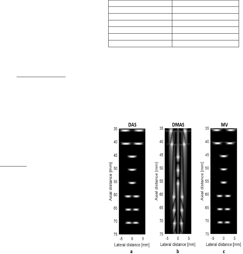
5.2 B-mode Image

After applying each method onto the received radio

frequency data. The images are then normalized by

itself, after that the envelope of the signal will be

extracted. A log compression is used with a dynamic

range of 60 dB. After passing through this process the

final image of each from the studied methods will be

show,

Figure 4: F-DMAS beamformer block-diagram.

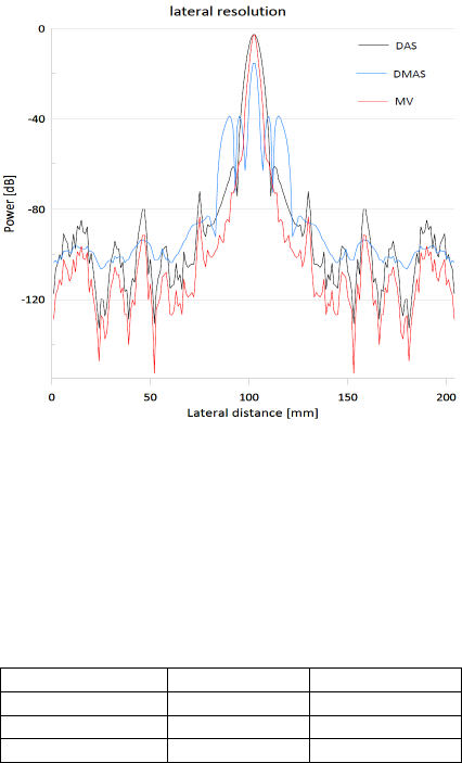
Figure 5: Lateral variation of DAS, DAMS and MV

The performance of the aforementioned techniques is

estimated using the Peak-Side-Lob and Full-Width at

Half Maximum (FWHM) values (PSL), we choice

randomly the depth of 57 mm for the evaluation in

this paper,

Table 2: FWHM and PSL od the different used techniques.

Parameters FWHM

(

)

PSL

DAS

1.53 -2.82

DMAS

0.98 -15.53

1.23 -2.88

6 CONCLUSION

From the lateral resolution we notice clearly that the

minimum variance beamforming shows the good

performance the main-lobe becomes very narrow as

long as the amplitude stays high however DAS

beamforming provides a good amplitude but the

main-lobe is still wide which gives a poor resolution

as we have already described

unfortunately, the DMAS technique shows a poor

performance given the time it takes to give the result.

although the main lobe is very narrow but note to the

huge loss in contrast due to the degradation in terms

of signal amplitude as well as the sidelobes which are

not well attenuated like the case of MV and DAS.

for this paper, the study was limited to the basic

aspect of its methods which can be improved as well

as the use of metrics like FWHM and PSL which

judges very well the different techniques possible in

this field.

REFERENCES

Hoskins, P. R., Martin, K., & Thrush, A. (2010). Diagnostic

ultrasound: Physics and equipment. Cambridge, UK:

Cambridge University Press (2nd edition).

Mehdi Haji Heidari Varnosfaderani, Babak

Mohammadzadeh, 2018. An Adaptive Synthetic

Aperture Method Applied to Ultrasound Tissue

Harmonic Imaging IEEE transactions on ultrasonics,

ferroelectrics, and frequency control, vol. 65, no. 4

B.M. Asl, A.M. Deylami, 2018. A Low Complexity

Minimum Variance Beamformer for Ultrasound

Imaging Using Dominant Mode Rejection, Ultrasonics

Volume 85, Pages 49-60

Jieming Ma and all, 2014. Ultrasound phase rotation

beamforming on multi-core DSP; Ultrasonics Volume

54, Issue 1, Pages 99-105

Jongin Park, Seungwan Jeon, Jing Meng, Liang Song, Jin

S. Lee, Chulhong Kim, (2016). “Delay-multiply-and-

sumbased synthetic aperture focusing in photoacoustic

microscopy,” J. Biomed. Opt. 21(3),036010, doi:

10.1117/1.JBO.21.3.036010.

Giulia Matrone and Al: High Frame-Rate, High Resolution

Ultrasound Imaging with Multi-Line Transmission and

Filtered-Delay Multiply And Sum Beamforming DOI

10.1109/TMI.2016.2615069, IEEE Transactions on

Medical Imaging

Jin Ho Sung and Jong Seob Jeong: Dual-/tri-apodization

techniques for high frequency ultrasound imaging: a

simulation study https://www.biomedical-engineering-

online.com/content/13/1/143

G. Matrone, A. S. Savoia, G. Caliano, G. Magenes, 2015.

“The Delay Multiply and Sum beamforming algorithm

in ultrasound B-mode medical imaging,” IEEE Trans.

Med. Imag., vol. 34, no. 4, pp. 940-949.

G. Matrone, A. S. Savoia, G. Caliano, G. Magenes, 2016.

“The “Ultrasound Plane-Wave Imaging with Delay

Multiply And Sum Beamforming and Coherent

Compounding,” Proc. IEEE Conf. Eng. Med. Biol.

Soc.(EMBC), Orlando, FL, pp. 3223-3226.

Nguyen, N. Q., & Prager, R. W. (2016). High-Resolution

Ultrasound Imaging With Unified Pixel-Based

Beamforming. IEEE Transactions on Medical Imaging,

35(1), 98–108.

Svetoslav Ivanov Nikolov_, Jacob Kortbek_ and Jørgen

Arendt Jensen Practical Applications of Synthetic

Aperture Imaging

Ali Mohades Deylami and Babak Mohammadzadeh, 2018.

Asl iterative: minimum variance beamformer with low

complexity for medical ultrasound imaging: World

Federation for Ultrasound in Medicine & Biology.

Acacio J. Zimbico, and Al, 2018. Joint Adaptive

Beamforming to EnhanceNoise Suppression for

Medical Ultrasound Imaging; World Congress on

Medical Physics and Biomedical Engineering.

Holfort, I. K., Gran, F., & Jensen, J. A. (2009). Broadband

minimum variance beamforming for ultrasound

imaging. IEEE Transactions on Ultrasonics,

Ferroelectrics and Frequency Control, Volume: 56,

Issue: 2;

Giulia Matrone, 2018. AlExperimental evaluation of

ultrasound higher-order harmonic imaging with

Filtered-Delay Multiply And Sum (F-DMAS) non-

linear beamforming; Ultrasonics 86 59–68

Jeff Powers, and Frederick Kremkau, 2011. Review

Medical ultrasound systems; The Royal Society

J. F. Synnevåg, 2008. “Adaptive beamforming for medical

ultrasound imaging,” Ph.D. thesis, Faculty

Mathematics and Natural Sciences, Univ. of Oslo, Oslo,

Norway.

B. Mohammadzadeh Asl and A. Mahloojifar, 2009. ”

Minimum Variance Beamforming Combined with

Adaptive Coherence Weighting Applied to Medical

Ultrasound Imaging,” IEEE Trans. Ultrason.

Ferroelect. Volume: 56, Issue: 9.

Carl-Inge Colombo Nilsen, 2010. “Wiener Beamforming

and the Coherence Factor in Ultrasound Imaging,”.

IEEE Transactions on Ultrasonics, Ferroelectrics, and

Frequency Control, vol. 57, no. 6.

J. A. Jensen, 1996. “Field: A program for simulating

ultrasound systems,” in 10th Nordicbaltic Conference

on Biomedical Imaging, vol. 4, supplement 1, part 1:

351–353. Citeseer,.