Forecasting River Water Quality using Autoregressive Integrated Moving
Average (ARIMA)
Dinna Yunika Hardiyanti
1
, Hardini Novianty
2
and Dinda Lestarini
3
1
Electronic Data Processing and Decision Support System Laboratory, Faculty of Computer Science, Universitas
Sriwijaya, Palembang, Indonesia
2
Faculty of Computer Science, Universitas Sriwijaya, Palembang, Indonesia
3
Database and Big Data Laboratory, Faculty of Computer Science, Universitas Sriwijaya, Palembang, Indonesia
Keywords:
Forecasting, ARIMA, Water Quality Parameters.
Abstract:
Water quality affects the level of public health and the welfare of society. So it is necessary to keep the water
clean. This study aims to predict the water quality of river X using the Arima method. The research uses the
degree of acidity (pH), COD, and BOD data from 2007 to 2018. The forecasting results show that pH is 7.44,
the COD value is 50.4184, and the BOD value is 3.310473. Therefore, in 2019, river X is in class III, which
is the river is for freshwater fish cultivation, livestock, or crop irrigation.
1 INTRODUCTION
Sustainable availability of clean water is a global
problem, including in Indonesia (Rahim and
Soeprobowati, 2019). Clean water vitally needs for
drinking, daily needs, agriculture, and also economic
needs, such as fishery and plantation. If water
quality decreases (contaminated), it will affect the
level of public health and the welfare of society
(Smiley and Hambati, 2019). Water quality control
is needed to reduce the risk of river water pollution
and the availability of sustainable clean water. The
Indonesian government issued regulations regarding
the use of clean water-based on the allocation into
four classes. Class I is for raw water of drinking
water. Class II is for infrastructure or water recreation
facilities, freshwater fish cultivation, livestock, water
for irrigating crops. Class III is for freshwater fish
cultivation, livestock, crops irrigation, while Class IV
is for irrigating crops only.
In this study, we used three parameters of river wa-
ter quality. These parameters are the degree of acidity
(pH), Chemical Oxygen Demand (COD), and Biolog-
ical Oxygen Demand (BOD). pH indicates the levels
of hydrographic ions contained in the water (Rahim
and Soeprobowati, 2019) (Waleed et al., 2019). pH
levels in the body affect the body’s metabolism and
ability to produce enzymes and hormones in the cen-
tral nervous system. COD parameters indicate the
need for oxygen to oxidize dissolved compounds and
organic particles in water (Chen et al., 2018) (Le
et al., 2018). The smaller the COD value of wa-
ter, the cleaner the water becomes. BOD shows the
oxygen demand needed by microorganisms to break
down dissolved and suspended organic substances in
water (Liang et al., 2018) (Spurr et al., 2018).
The Indonesian government states that clean wa-
ter has a pH between 7 and 9. If the pH more than
nine and less than seven water is polluted. COD pa-
rameters have different values for each class. Class I
pH value of 10 mg / l, class II of 25 mg / l, class III of
50 mg / l, while class IV 100. This value indicates the
oxygen needed by organic particles to carry out oxi-
dation. So the higher the value of COD can be said
the water is increasingly polluted. Because the level
of oxygen needed to carry out oxidation is higher than
usual. BOD parameter values for each class differed,
namely in class I BOD values of 2 mg / l, class II by 3
mg / l, class III by 6 mg / l, while grade IV by 12 mg /
l. This value is different because the BOD value indi-
cates the amount of oxygen needed by microorganism
for suspended organic substances. So that if the BOD
value indicates more than 12 mg / l, that river water is
polluted.
This study aims to predict river water quality by
examining river water data. Research data used are
river X measurement data. Wheres X river is a river
located on the island of Java, Indonesia. This river
is used to meet the needs of clean water by residents.
The prediction results will be used to determine wa-
158
Hardiyanti, D., Novianty, H. and Lestarini, D.
Forecasting River Water Quality using Autoregressive Integrated Moving Average (ARIMA).
DOI: 10.5220/0009907201580163
In Proceedings of the International Conferences on Information System and Technology (CONRIST 2019), pages 158-163
ISBN: 978-989-758-453-4
Copyright
c
 2020 by SCITEPRESS – Science and Technology Publications, Lda. All rights reserved

ter pollution prevention policies. The method used
is a time series that analyses data based on a certain.
ARIMA time series method analyses stationary and
non-stationary data to make predictions. Its accuracy
can reach 91.85% (Arya and Zhang, 2015) (York and
Gernand, 2017). So the ARIMA method can make
more accurate predictions.
2 LITERATURE REVIEW
2.1 Time Series
Time series analysis is a set of observations with uni-
form observation. The time-series analysis on the as-
sumption that the values of a data set are historically
consecutive with the same intervals between obser-
vations (Ivanovi
´
c and Kurbalija, 2016). The purpose
of using time series analysis is to identify the charac-
teristics of the phenomena observed sequentially and
predict the value that will occur in the time series. To
achieve these two objectives requires the identifica-
tion of the data pattern of the observation time se-
ries. So that its relationship with other phenomena
can show. Thus, the identified time series patterns
can be extrapolated to predict future events. In gen-
eral, the time-series pattern can describe two primary
components, which are trends and seasonality.
2.2 Autoregressive Integrated Moving
Average (ARIMA)
The Autoregressive Integrated Moving Average
(Arima) method, commonly called the Box-Jenkins
method is a method developed by George Box and
Gwilym Jenkins in 1970 (Arya and Zhang, 2015).
The Arima method is a method used for short-term
forecasting. The use of the ARIMA method in short-
term forecasting is very appropriate to use because the
ARIMA method has a very accurate accuracy (Arya
and Zhang, 2015). Also, determine an excellent sta-
tistical relationship between variables to be predicted
with the value used for forecasting. While for long-
term forecasting, the accuracy of forecasting is not
good. Usually, the forecast value will tend to be con-
stant for a reasonably long period.
In solving problems from a time series data using
pure AR / ARIMA (p,0,0), pure MA / ARIMA (0,0,q),
ARMA / ARIMA (p,0,q) or ARIMA (p,d,q) through
several stages, namely identification, parameter es-
timation, diagnostic testing and forecasting applica-
tion. Model groups included in the ARIMA method
are (Tauryawati and Irawan, 2014).
1. Autoregressive Model (AR)
The assumption held by this model that data in-
fluenced by past data. Called the Autoregressive
model because in this model it is regressed against
the previous values of the variable itself. The au-
toregressive model with the order p shortened to
AR (p) or ARIMA (p, 0,0). The general equation
of the AR model (p,0,0) in equation 1.
Z
t
= µ + Ø
1
Z
t−1
+ Ø
2
Z
t−2
+ ... + Ø
p
Z
t− p
+ a
t
(1)
Wheres,
Z
t
= stationary time series
µ = constant
Z
t− p
= independent variable
Ø
p
= coefficient of the autoregressive at p
a
t
= error value at t
2. Moving Average Model (MA)
The general form of the moving average of the
order q (MA (q)) or ARIMA (0.0, q) shown in
equation 2.
Z
t
= µ + a
t
–θ
1
a
t−1
–θ
2
a
t−2
–...–θ
q
a
t−q
(2)
Wheres,
Z
t
= stationary time series
µ = constant
a
t−q
= independent variable
θ
q
= coefficient of the autoregressive at p
a
t
= error value at t
3. ARMA
The Autoregressive Moving Average (ARMA)
model is a combined model of the Autoregressive
(AR) and Moving Average (MA). This model has
the assumption that the previous data influence
current data. The general form of ARMA shown
in equation 3.
Z
t
= µ + Ø
1
Z
t−1
+ ... + Ø
p
Z
t− p
+
a
t
–θ
1
a
t−1
–...–θ
q
a
t−q
(3)
Wheres, Z
t
= stationary time series µ = constant
Z
t− p
= independent variable Ø
p
= coefficient of
the autoregressive at p a
t−1
= independent vari-
able θ
q
= coefficient moving average parameter
a
t−q
a
t
= error value at t
4. ARIMA
The Integrated Moving Average Autoregressive
Model (ARIMA) is used based on the assump-
tion that the time series data used must be station-
ary, meaning that the average variation of the data
Forecasting River Water Quality using Autoregressive Integrated Moving Average (ARIMA)
159

in question is constant. However, several things
happen when data is not stationary. In overcom-
ing this unstable data, a differencing process so
that the data becomes stationary. The Autoregres-
sive (AR), Moving Average (MA), Autoregressive
Moving Average (ARMA) models are not able to
explain the meaning of the difference. A mixed
model called the Autoregressive Integrated Mov-
ing Average (ARIMA), or ARIMA (p,d,q) thus
becomes more effective in explaining the differ-
encing process. In this model, the stationary se-
ries is a linear function between past value with
present value and the past error. The general form
of ARIMA shown in equation 4.
φ
p
(B)D
d
Z
t
= µ + θ
q
(B)a
t
(4)
Wheres, φ
p
= coefficient of the autoregressive at p
θ
q
= coefficient moving average parameter a
t−q
B
= backshift operator D = differencing µ = constant
a
t
= error value at t p = degree of autoregressive d
= differencing process level q = degree of moving
an average
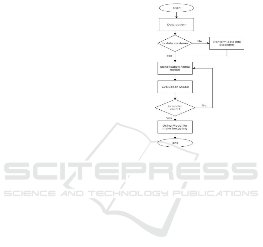
3 DATA ANALYSIS METHOD
ARIMA can make a forecast using stationery and
non-stationery data (Arya and Zhang, 2015). So, the
first step is to analyze data patterns. This analysis is
needed to find out stationary or non-stationary data.
If data not-stationer, it will be transformed into sta-
tioner data before make analysis forecast. Flow chart
of forecasting data using ARIMA show Figure1.
Identification of data patterns shows from Auto-
correlation (AC) and Partial Correlation (PAC) graph.
Another way can also use the root test to see the Aug-
mented Dickey-Fuller (ADF) value. Stationery data
has an ADF absolute value is higher than the test crit-
ical values. If the ADF value is smaller than the crit-
ical value, then do difference level 1 and do the root
test again. If the root test results for differencing one
show stationary data. Then the identification of the
Arima model identification can be made with differ-
encing 1. However, if the data is not stationary, then
do difference level 2. Then do the root test for differ-
encing level 2.
space
Figure 1: Flow chart of forecasting data using Arima.
AC and PAC graphs predict p and q ordo can. If
the AC chart, there is a graph that crosses the line
then we have an MA candidate 1. in the PAC graph
there is a bar that crosses the line, then we get a AR 1
candidate. Then the D coefficient is the differencing
level for converting data into stationary data
The selected Arima model has the smallest values
of the Akaide Info Criterion (AIC) and Schwarz crite-
rion (SC). Than developing ARIMA equation model
based on the coefficient, AR, MA, ARMA values. For
evaluation chosen model, in this paper, use residual
test. Residual test show autocorrelation problem in
Grafik AC, PAC and QStat values. A good model suc-
cessfully resolves the autocorrelation problem. It can
show from the Q-stat value, which is not significant
in each lag.
The best model chosen is used to make fore-
casting. The resulting model accuracy show from
the Mean Absolute error (MAE) value. The more
the MAE value approaches 0, the more accurate the
model. Because the MAE value shows the difference
between predictions with real values.
CONRIST 2019 - International Conferences on Information System and Technology
160

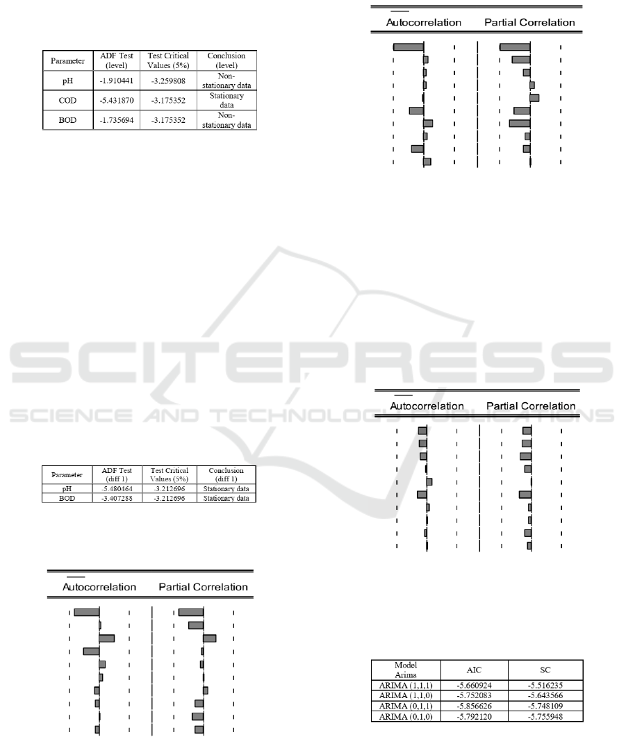
4 RESULT AND DISCUSSION
This study uses the measurement data of river water
pollution from 2007 to 2018 in on one of the rivers
in Java. Measurement data are analyzed to determine
data patterns. The data is analyzed using the root test.
The results of the data analysis shown in Figure 2.
Figure 2: Stationarity Test Results Using The Augmented
Dicky Fuller Test Method.
Based on Figure 2, the pH and BOD parame-
ter data are non-stationary data, because the absolute
ADF value is smaller than the critical test value at a
5% confidence level. So the pH and BOD values are
transformed using difference level 1. The COD pa-
rameter data is stationary because the absolute ADF
is higher than the critical test value. So the difference
value (D) is 0.
Analysis of pH and BOD parameters using differ-
ent level 1 in Figure 3. The results of the data analysis
show that parameter pH and BOD data are stationary.
It can show that the absolute ADF value is higher than
the critical test value for the two parameters. So the
difference value for pH and BOD parameters is 1.
The next step is to determine the possibility of p
and q ordo using AC and PAC tests. These result AC
and PAC analysis for parameter pH (Figure 4), COD
(Figure 5), and BOD (Figure 6).
Figure 3: Stationary test results of pH and BOD parame-
ters after being transformed Using Augmented Dicky Fuller
Test Method.
Figure 4: AC and PAC Analysis for pH Parameter
AC and PAC graphs of pH parameters (Figure 4)
show no bar crossing the line. So that the order p and
q are 0 or 1. Besides, the value of D defines as 1.
So that the possibility of the Arima model that will
be used is ARIMA (1,1,1), ARIMA (1,1,0), ARIMA
(0,1,1) or ARIMA (0,1,0).
Figure 5: AC and PAC Analysis for COD Parameter
AC and PAC graphs show COD parameters (Fig-
ure 5) show no bar crossed the line. So that the order
p and q are 0 or 1. Besides that, the D value defined as
0. So that the possibility of the Arima model that will
show is ARIMA (1,0,1), ARIMA (1,0,0), ARIMA
(0,0,1) or ARIMA (0,0,0).
AC chart and PAC for BOD parameters (Figure 6)
show no bar crossed the line. So that the order p and q
are 0 or 1. The value of D is 1. So that the possibility
of the Arima model that will be used is Arima (1,1,1),
Arima (1,1,0), Arima (0,1, 1) or Arima (0,1,0)
Figure 6: AC and PAC Analysis for BOD Parameter
The possibility of the Arima model on each pa-
rameter was analyzed to find out AIC and SC values.
The model chosen has the smallest AIC and SC val-
ues.
Figure 7: AIC and SC values for pH parameter.
In Figure 7 shows ARIMA (0,1,1) has the smallest
AIC and SC values of -5.856626 and -5.748109. So,
pH parameters using the ARIMA (0,1,1).
Forecasting River Water Quality using Autoregressive Integrated Moving Average (ARIMA)
161

space
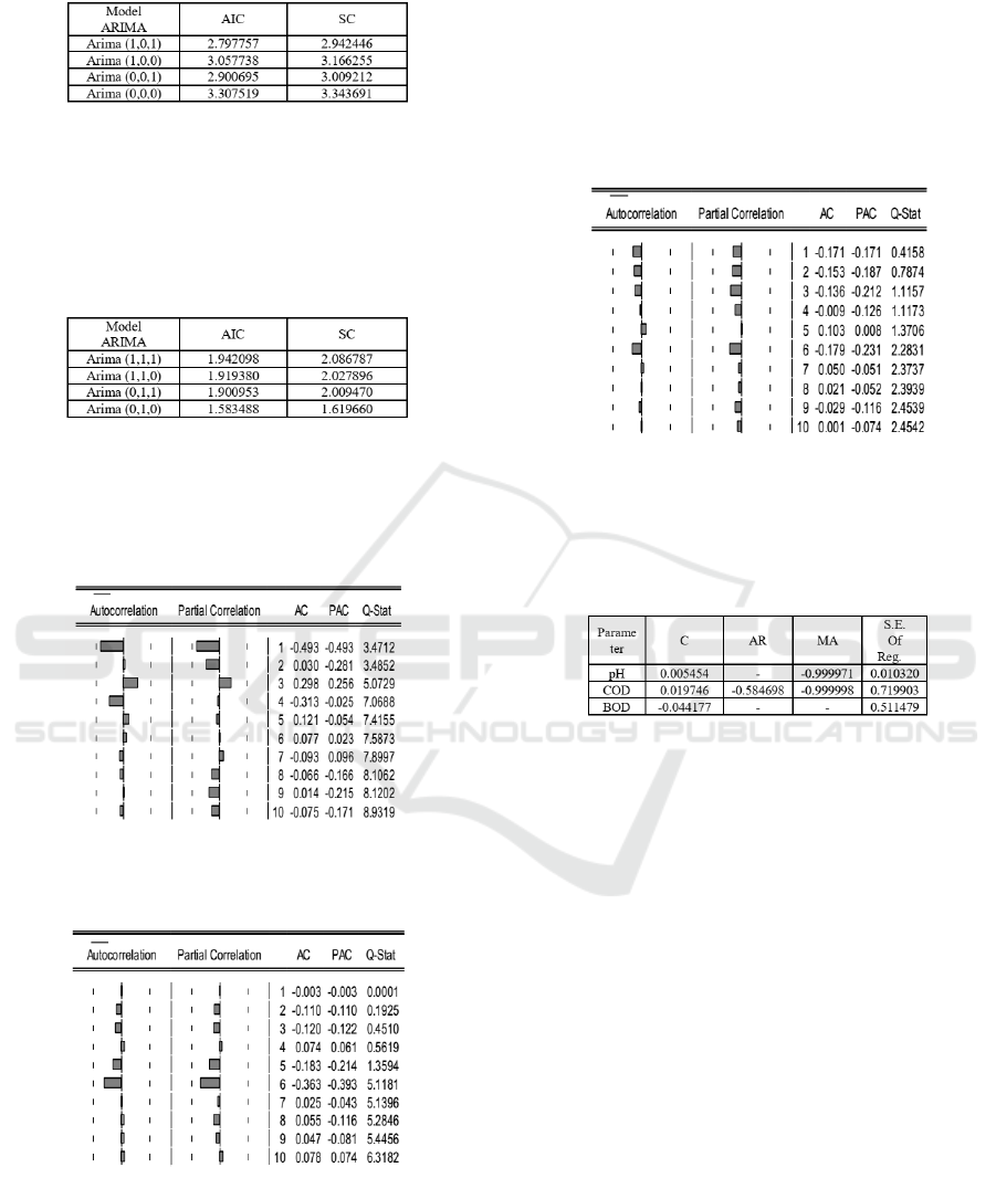
Figure 8: AIC and SC values for COD parameter.
In Figure 8 shows ARIMA (1,0,1) has the smallest
AIC and SC values of 2.797757 and 2.942446. So for
COD parameters using the ARIMA (1,0,1).
In Figure 9 shows ARIMA (0,1,0) has the smallest
AIC and SC values of 2. 1.583488 and 1.619660. So
for BOD parameters using the ARIMA (0,1,0).
Figure 9: AIC and SC values for BOD parameter.
The model selected for each parameter validated
by residual white noise test. This test aims to deter-
mine whether the model can solve the autocorrelation
problem or not.
Figure 10: Residual cost test results for pH parameter
Figure 11: Residual cost test results for COD parameter
Figure 10 shows the results of the residual white
noise test for pH parameters. ARIMA (0,1,1) for the
pH parameter. Figure 11 shows the results of the
residual white noise test for COD parameters. Fig-
ure 12 shows the results of the residual white noise
test for BOD parameters. In all three pictures, no bar
crosses the line. So, the ARIMA (0,1,1) for the pH
parameter, ARIMA (1,0,1) for the COD parameter,
and ARIMA (0,1,0) for the BOD parameter can solve
the autocorrelation problem. So that Arima equation
can be built based on the coefficient values, AR, MA
and S.E of Regression from each Arima model for the
three parameters.
Figure 12: Residual cost test results for BOD parameter
Figure 13 shows the analysis result coefficient,
AR, MA and SE of Regression for ARIMA (0,1,1)
for the pH parameter, ARIMA (1,0,1) for the COD
parameter, and ARIMA (0,1,0) for the BOD.
Figure 13: Coefficient AR, MA and ARMA values.
Forecasting equation for pH parameters using
ARIMA (0,1,1) is in equation 1. Forecasting equa-
tion for COD parameters using ARIMA (1,0,1) is in
equation 2. Forecasting equation for BOD parameters
using ARIMA (0,1,0) is in equation 3.
Z
t
= 0.005454 + 0.010320a
t−q
− (−0.999971) (5)
Z
t
= 0.0.019746 + (−0.584698)a
t− p
−
(−0.999998a
t−q
) + 0.999998 (6)
Z
t
= −0.044177Z
t
+ 0.511479a
t−1
(7)
The forecast value of pH in 2019 is 7.45 with the
MAE coefficient of 0.008649 based on equation 1. the
forecast value of COD in 2019 is 50.4184 with the
MAE coefficient of 0.552897 from equation 2. the
forecast value of BOD in 2019 is 3.310473 with the
MAE coefficient of 0.414456 from equation 3.
CONRIST 2019 - International Conferences on Information System and Technology
162

5 CONCLUSIONS
The prediction of water quality on river X in 2019
for the pH parameter is 7.45, the COD parameter is
50.4184, and the BOD parameter is 3.310473. Thus
in 2019, river X water is in class III. X river water is
predicted not to use as raw material for drinking wa-
ter, only for freshwater fish cultivation, livestock, crop
irrigation. So the government must make policies and
plan for pollution prevention on river X. So that in the
future river X can be used as raw material for drinking
water and other activities.
REFERENCES
Arya, F. K. and Zhang, L. (2015). Time series analysis
of water quality parameters at stillaguamish river us-
ing order series method. Stochastic environmental re-
search and risk assessment, 29(1):227–239.
Chen, J., Liu, S., Qi, X., Yan, S., and Guo, Q. (2018). Study
and design on chemical oxygen demand measurement
based on ultraviolet absorption. Sensors and Actua-
tors B: Chemical, 254:778–784.
Ivanovi
´
c, M. and Kurbalija, V. (2016). Time series anal-
ysis and possible applications. In 2016 39th Inter-
national Convention on Information and Communi-
cation Technology, Electronics and Microelectronics
(MIPRO), pages 473–479. IEEE.
Le, G., Yang, H., and Yu, X. (2018). Improved uv/o3
method for measuring the chemical oxygen demand.
Water Science and Technology, 77(5):1271–1279.
Liang, Q., Yamashita, T., Yamamoto-Ikemoto, R., and
Yokoyama, H. (2018). Flame-oxidized stainless-steel
anode as a probe in bioelectrochemical system-based
biosensors to monitor the biochemical oxygen de-
mand of wastewater. Sensors, 18(2):607.
Rahim, A. and Soeprobowati, T. R. (2019). Water pollution
index of batujai reservoir, central lombok regency-
indonesia. Journal of Ecological Engineering, 20(3).
Smiley, S. L. and Hambati, H. (2019). Impacts of flood-
ing on drinking water access in dar es salaam, tan-
zania: implications for the sustainable development
goals. Journal of Water, Sanitation and Hygiene for
Development, 9(2):392–396.
Spurr, M. W., Eileen, H. Y., Scott, K., and Head, I. M.
(2018). Extending the dynamic range of biochemi-
cal oxygen demand sensing with multi-stage micro-
bial fuel cells. Environmental Science: Water Re-
search & Technology, 4(12):2029–2040.
Tauryawati, M. L. and Irawan, M. I. (2014). Perbandin-
gan metode fuzzy time series cheng dan metode box-
jenkins untuk memprediksi ihsg. Jurnal Sains dan
Seni ITS, 3(2):A34–A39.
Waleed, A. K., Kusuma, P. D., and Setianingsih, C. (2019).
Monitoring and classification system of river wa-
ter pollution conditions with fuzzy logic. In 2019
IEEE International Conference on Industry 4.0, Ar-
tificial Intelligence, and Communications Technology
(IAICT), pages 112–117. IEEE.
York, J. C. and Gernand, J. M. (2017). Evaluating the
performance and accuracy of incident rate forecasting
methods for mining operations. ASCE-ASME Journal
of Risk and Uncertainty in Engineering Systems, Part
B: Mechanical Engineering, 3(4).
Forecasting River Water Quality using Autoregressive Integrated Moving Average (ARIMA)
163