Data Panel Modelling with Fixed Effect Model (FEM) Approach to

Analyze the Inﬂuencing Factors of DHF in Pasuruan Regency

Achmad Faridz Jauhari

, Yoyon K. Suprapto

and Achmad Mauludiyanto

Department of Electrical Engineering Institut Teknologi Sepuluh Nopember Surabaya, Indonesia

Keywords:

Panel Data, Fixed Effect Model, Regression Analysis, Ordinary Least Square, Dengue Hemorrhagic Fever.

Abstract:

Dengue Hemorrhagic Fever (DHF) is one of the endemic diseases caused by the bites of Aedes mosquitoes

which are infected with the dengue virus. This disease can cause death. The DHF mortality rate in Pasu-

ruan Regency is high (above 1% per year) in the last four years. Therefore, this study aimed to ﬁnd a model

that can explain the inﬂuencing factors of DHF incidence. The variables used were the number of DHF pa-

tients(Y), waste volume(X

), rainy days(X

), health facilities(X

), temperature(X

), number of high-educated

population(X

), population density(X

), and rainfall(X

). The data used were ranging from 2015 to 2018 and

obtained from several agencies in Pasuruan Regency. In this study, the method used was the Panel Data Re-

gression with Fixed Effect Model approach. The results of the model showed R

: 0.804 meaning that the

seven variables were able to explain the effect on the incidence of DHF by 80.4% while the remaining 19.6%

was inﬂuenced by other unknown variables. Of the seven predictor variables, there are six variables that have

a signiﬁcant effect consist of Waste Volume, Health Facilities, Temperature, Number of High-Educated Popu-

lation, Population Density, and Rainfall. Henceforth, future DHF prevention and control policies can be more

emphasized on these factors.

1 INTRODUCTION

Dengue hemorrhagic fever (DHF) is a disease caused

by the dengue virus and is transmitted by Aedes ae-

gypti and Aedes albopictus mosquitos. Both types of

mosquitoes are found in all corners of Indonesia, ex-

cept in places with altitudes above 1000 masl (meters

above sea level) (Arsin, 2013). The symptoms pa-

tients is a high fever for 2-7 days (38-400°C). At the

acute level, this disease can cause death. Besides that,

DHF can appear throughout the year and can affect all

age groups (Kemenkes, 2017).

Indonesia is the country which has the highest

DHF cases in Southeast Asia (Kemenkes, 2010). In

the last ﬁve years, the highest number of dengue cases

was occurred in 2016 reaching up to 204,171 cases

with 1,598 deaths. The number of dengue cases in

2016 increased by 57.5% compared to the number

of dengue cases in 2015 which was 129,650 cases.

The number of DHF deaths in 2016 also worsens by

49.2% compared to the number of deaths in 2015

which was only 1,071 people. It was also reported

that the Incident Rate (IR) in 2015 increased from

50.75 to 78.85 per 100,000 population. However, the

Case Fatality Rate (CFR) has decreased from 0.83%

in 2015 to 0.78% in 2016. DHF has spread in 34

provinces and 463 districts/cities in Indonesia (Ke-

menkes, 2017).

Pasuruan Regency is one of the regions in East

Java where its DHF mortality rate is above 1% in this

past four years. Since 2015, DHF is determined as an

Extraordinary Situation and as a result, the efforts to

control DHF were carried out intensively. Based on

the data released by the Public Health Ofﬁce of Pa-

suruan Regency, the number of DHF cases in 2015

was 686 cases with 28 deaths whereas, in 2016, the

number of DHF cases increased by 11% to 764 cases

with a total death of 27 people. In 2017, the number

of DHF cases decreased by 59% to 317 cases with

13 deaths and continued to decline by 38% with four

deaths in 2018. The Incident Rate (IR) of DHF in

2015 was 43.31 per a 100,000 population while the

Case Fatality Rate (CFR) was 4.1%. In 2016, the

IR increased to 48.23 per a 100,000 population while

the CFR dropped to 3.5%. On the other hand, in

2017, the IR decreased to 19.75 per 100,000 popula-

tion while the CFR increased to 4.1%. In 2018, the IR

was 11.90 per 100,000 population while the CFR was

2.1%. Based on the above data, the mortality/Case

Fatality Rate of DHF in Pasuruan for the past four

224

Jauhari, A., Suprapto, Y. and Mauludiyanto, A.

Data Panel Modelling with Fixed Effect Model (FEM) Approach to Analyze the Inﬂuencing Factors of DHF in Pasuruan Regency.

DOI: 10.5220/0009881702240232

In Proceedings of the 2nd International Conference on Applied Science, Engineering and Social Sciences (ICASESS 2019), pages 224-232

ISBN: 978-989-758-452-7

years is included in the high category (CFR ¿ 1%)

(Kemenkes, 2017).

The spread of DHF in Indonesia is inﬂuenced by

many factors such as climate, community behaviour,

environment, as well as demographic and socioeco-

nomic conditions (Arsin, 2013). The climate factors

include temperature, rainfall, rainy days, humidity,

and wind speed; behavioural factor is basically a per-

son’s response towards stimuli that is related to illness

and disease including knowledge, actions, and beliefs

associated with DHF, availability of health resources,

adequate and affordability of health facilities, com-

munity support, as well as the concern from govern-

ment and health workers; environmental factors are

the number of places or containers of DHF vector pro-

liferation; demographic factors consist of the popula-

tion density and population mobility; socio-economic

factors are the level of education, employment, and

the number of family members. Of the factors men-

tioned above, knowing which of the factors that have

a signiﬁcant effect on DHF is very important so that

future efforts to prevent and control DHF can be done

more effectively and efﬁciently.

Modelling is a method that can be used to de-

termine the factors that have a signiﬁcant effect on

DHF in Pasuruan Regency. This study aimed to ﬁnd

a model that is able to explain the inﬂuencing fac-

tors of DHF in 21 sub-districts of Pasuruan within the

period of 2015 to 2018. Different regional character-

istics in each sub-district are thought to inﬂuence the

incidence of DHF. By that, this study used Panel Data

structure. There has never been a research which ex-

amined the factors of DHF in Pasuruan Regency so

that the results of this modelling are expected to be

used as early warnings or basis for the formulation of

strategic policies to prevent and eradicate DHF in the

future.

Several studies related to the analysis of DHF have

been done before. Research conducted by (Ariani,

2018) used the Negative Binomial regression model

to produce variables that signiﬁcantly inﬂuence DHF,

namely population density, number of health workers

and rainfall. Subsequent research by (Rustiani, 2017)

using multiple linear regression resulted in R

values

of 67 percent, signiﬁcant variables included popula-

tion density, rainfall and larva free index. Research

conducted by (Rasmanto, 2016) using Linear Regres-

sion resulted in R

values of 24.1 percent, variables

that had a signiﬁcant effect consisted of air temper-

ature and relative humidity. The study by (Hasirun,

2016) used a Spatial regression model with spatial

error resulting in R

values of 43.34 percent, sig-

niﬁcant variables covering rainfall, health facilities,

the percentage of PHBS houses, and the percentage

of healthy houses. Subsequent research by (Martha,

2015) used panel data regression with a ﬁxed effect

model approach resulted in R

values of 72,76 per-

cent, signiﬁcant variables included population den-

sity, population mobility, the average age of DHF pa-

tients, and the number of DHF patients in the previous

time period. Based on these studies we use several

variables that have been used previously namely pop-

ulation density, rainfall, rainy days, temperature, and

the number of health facilities. Then we add two new

variables namely the waste volume and the Number

of High-Educated Population.

2 LITERATURE REVIEW

2.1 Panel Data

Panel Data is a collection of data consisting of cross-

section data and time series data. Time series data

usually includes one individual observed in a certain

period of time while cross-section data is obtained

from several individuals observed in a certain period

of time. Therefore, it can be said that the Panel Data

presents larger and more informative data and gener-

ates a greater degree of freedom. The general form of

Panel Data regression models can be seen in Equation

1 (Hsiao, 2003; I. et al., 2017).

= α

+ β

+ ε

(1)

2.2 Estimation of Panel Data

Regression Model

In making parameter estimation, the model depends

on the assumptions about intercepts and slope coef-

ﬁcients. Using Panel Data allows different intercepts

and slope coefﬁcients to occur in each individual and

each time period. In this concept, there are three ap-

proaches that can be used, namely CEM (Common

Effect Models), FEM (Fixed Effect Model) and REM

(Random Effect Models) (Widarjono, 2013; I. et al.,

2017)

Data Panel Modelling with Fixed Effect Model (FEM) Approach to Analyze the Inﬂuencing Factors of DHF in Pasuruan Regency

225

2.2.1 CEM (Common Effect Models)

The approach with CEM model assumes that inter-

cepts and slope coefﬁcients have the same value for

all individuals at all time periods. In other words, this

model ignores individual dimensions and time. The

equation of CEM model is illustrated in this follow-

ing Equation 2.

= α + β

+ ε

(2)

2.2.2 FEM (Fixed Effect Model)

This approach believes that differences in character-

istics between individuals are represented in the in-

tercepts. Thus, intercepts for each individual will be

different but the slope coefﬁcients remain constant at

all time periods. Equation 3 below presents the equa-

tion of FEM model.

= α

+ β

+ ε

(3)

2.2.3 REM (Random Effect Models)

In REM, the differences in individual characteristics

are accommodated by error terms. Error terms may

correlate between individuals and between times. For

more details, the equation of REM model is formu-

lated in Equation 4.

= α + β

(4)

α is the mean of intercept from error terms cross

section and time series. W

: µ

+ ε

where µ

is the

random error cross section deviation, which explains

the differences between individuals and each other.

2.3 Selection of Panel Data Regression

Model

In choosing the model that will be used to manage

Panel Data, several tests need to be done, namely:

2.3.1 Chow Test

Chow Test is used to choose a better model between

CEM and FEM (Greene, 2000). The hypothesis in the

Chow Test can be written as follows.

: α

= α

= ·· · = α

= 0 (CEM)

: minimumo f oneα

6= 0 (FEM)

Next, the equation for Chow Test Statistics is:

count

(RRSS −URSS)/(N − 1)

URSS/(nT − n −K)

(5)

Description: RRSS: restricted residual sum of

square CEM URSS: unrestricted residual sum of

square FEM n: number of individuals(cross section)

T: time periods (Time Series) If the value of F

ount ≥

able = F

(n−1,nT −n−K)

or p − value ≤ 0.05, then hy-

pothesis H

is rejected. This means that FEM is a

better model than CEM.

2.3.2 Hausman Test

Hausman test is used to choose a better model be-

tween FEM and REM (Baltagi, 2010; Sutikno et al.,

2017). The hypothesis in the Hausman Test is as fol-

lows.

: correlation(µ

) = 0(REM)

: correlation(µ

) 6= 0(FEM)

This following equation 6 displays the Hausman

Test Statistics.

W =(

FEM

−

REM

)

[var(

FEM

−

REM

)]

−1

(

FEM

−

REM

)

(6)

If the value of W ≥ χ

table

= χ

(a,K)

or p − value ≤

0.05, then hypothesis H

rejected, meaning that FEM

is a better model than REM. But if the value of W <

table

= χ

(a,K)

or p − value > 0.05, then hypothesis

, is accepted. This points out that the best model

between FEM and REM is REM.

2.3.3 Lagrange Multiplier Test

LM Test is used to choose a better model between

CEM and REM. LM Test does not need to be done

if FEM is found to be the best in the Chow Test and

Hausman Test. This test is only done when the best

model found in the Chow Test is FEM whereas, in the

Hausman Test, the best model is REM. These are the

hypothesis in the LM test:

: σ

= 0(CEM).

: σ

6= 0(REM).

In details, the statistics of LM Test can be under-

stood through Equation 7 (Widarjono, 2013) below.

LM =

2(T − 1)

(

i=1

(T ˆe

)

i=1

t=1

ˆe

− 1)

(7)

Description:

n:number of individuals

T:time period

ˆe:error on CEM

ICASESS 2019 - International Conference on Applied Science, Engineering and Social Science

226

Hypothesis H

is rejected if the value of LM ≥

table

= χ

(a,K)

or p − value ≤ 0.05. This indicates that

REM is a better model than CEM. Otherwise, if the

value of LM < χ

table

= χ

(a,K))

or p − value > 0.05,

then the hypothesis H

is accepted which means that

the correct model between the two models is CEM.

2.3.4 Classical Assumptions Test

To get the estimator of the parameter model in the

CEM and FEM approach, Ordinary Least Square

(OLS) method is used. The classical assumption is

done to get the best OLS estimator known as BLUE

(Best Linear Unbiased Estimator). Classical assump-

tion tests include 1. Multicollinearity Test, 2. Nor-

mality Test, 3. Heteroscedasticity Test, and 4. Au-

tocorrelation Test. From all the four tests, only test

3 and 4 that must be met to obtain the best estimator

(BLUE) (Gujarati, 2004).

2.3.5 Multicollinearity Test

One of the assumptions used in OLS is the absence of

a strong relationship between predictor variables. The

presence of multicollinearity makes the model to have

a large variant (Widarjono, 2013)). However, multi-

collinearity can still produce BLUE estimators. One

way to detect multicollinearity is to use the sample of

correlation coefﬁcient (Gujarati, 2004; Sutikno et al.,

2017). The sample of correlation coefﬁcient is shown

in the next Equation 8.

(8)

If the correlation coefﬁcient is > 0.85, then it

is suspected that multicollinearity occurred in the

model. Conversely, if the correlation coefﬁcient is

≤ 0.85, it is assumed that the model did not contain

multicollinearity (Widarjono, 2013).

2.3.6 Normality Test

This assumption test is optional, but it is better if in-

cluded in an effort to get a good OLS estimator. The

hypotheses in this test are:

: E(ε

) = 0(error, distributed normally)

: E(ε

) = 0(error, not distributed normally)

The Normality Test Statistics adopted the Jarque-Bera

formula as we can see in this following Equation 9

(Gujarati, 2004)).

JB = NT (

− 3)

)

(9)

Description,

: slope(Skewness)

: height(kurtosis)

If the value of JB < χ

tabel

= χ

(a,2)

or p − value >

0.05, then hypothesis H

is accepted. This clariﬁes

that the error is normally distributed.

2.3.7 Heteroscedasticity Test

The assumption that the error variant has a constant

(homoscedastic) nature is very important to produce

the best OLS estimator. The Heteroscedasticity Test

hypothesis is:

error does not contain heteroscedasticity

error contain heteroscedasticity

Glejser Method is used for the Heteroscedastic-

ity Test Statistics, which is by regressing the abso-

lute value of the error with its independent variable

(Widarjono, 2013). If β

is not signiﬁcant in t-test

or the Prob value is> 0.05, then hypothesis H

is ac-

cepted. This explains that the error did not contain

heteroscedasticity or was constant.

2.3.8 Autocorrelation Test

This assumption test is used to see if there is no serial

correlation on the error. This test is crucial to get a

BLUE OLS estimator. One way to detect autocorre-

lation is to use a Durbin Watson test method. These

are the hypothesis for the autocorrelation test in this

study:

: Cov(ε

,ε

i,t−1

) = 0 (no autocorrelation)

: Cov(ε

,ε

i,t−1

) 6= 0 (there is autocorrelation)

The statistics of the Durbin Watson autocorrela-

tion test can be seen in equation 10 (Gujarati and P,

2010).

DW =

i=1

t=2

(ε

− ε

i,t−1

)

i=1

t=2

(10)

Data Panel Modelling with Fixed Effect Model (FEM) Approach to Analyze the Inﬂuencing Factors of DHF in Pasuruan Regency

227

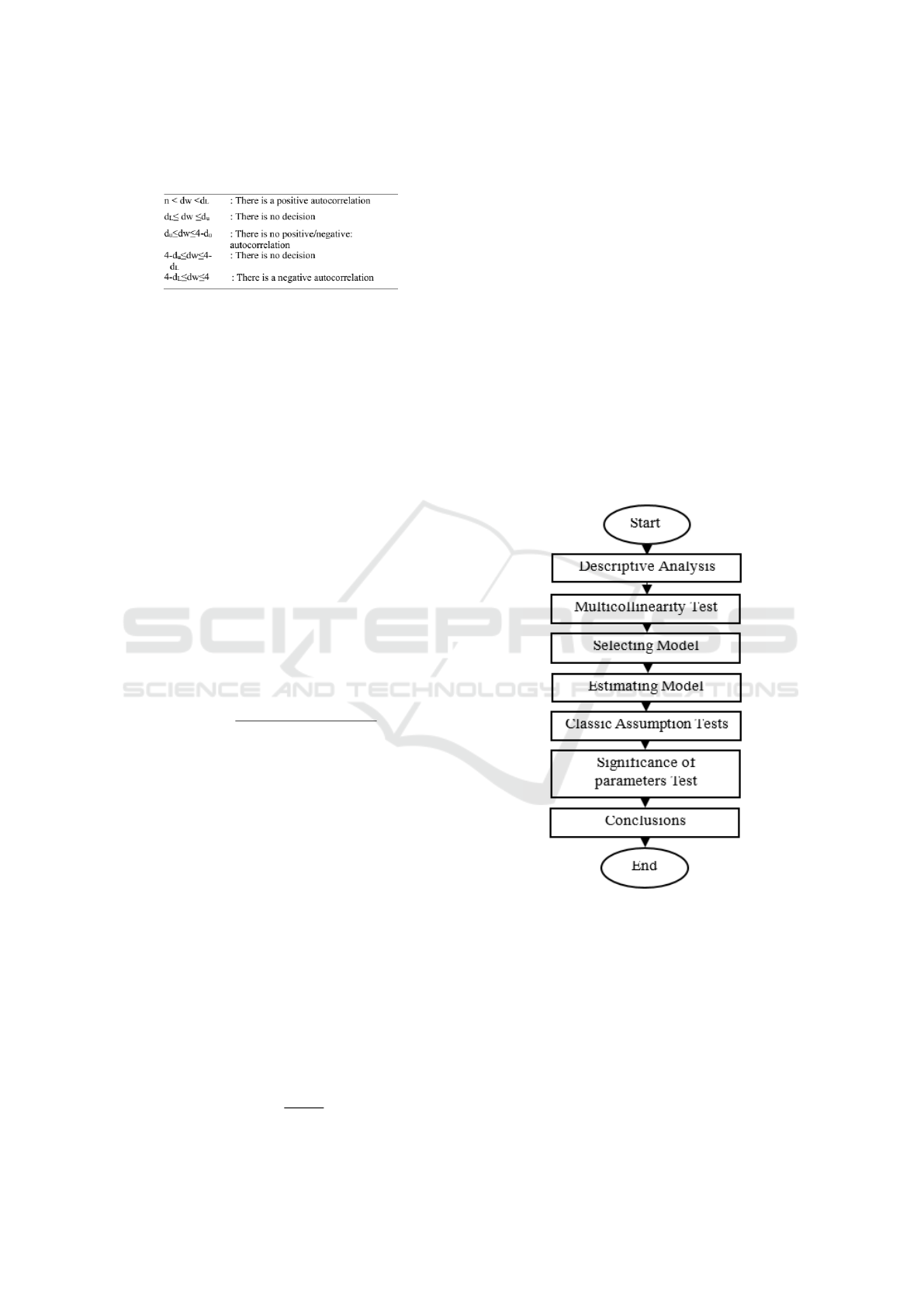
Figure 1 below presents the critical value in the

autocorrelation test:

Figure 1: Autocorrelation critical value of durbin watson

justiﬁed.

2.3.9 Signiﬁcance Test of Regression Parameters

The parameter signiﬁcance test is used to ﬁnd out the

level of inﬂuence that the predictor variable has on

the response variable. There are two tests carried out,

namely simultaneous test and partial test.

2.3.10 Simultaneous Test

A simultaneous test is applied to determine the ef-

fect of predictor variables on the response variable

together. The simultaneous test hypothesis is as fol-

lows.

: β

= β

= ··· = β

= 0 (all predictor variables

have no effect on the response variable)

:minimum of one β

6= 0 (there is at least one

predictor variable that affects the response vari-

able)

count

/(n + K − 1)

(1 − R

)/(nT − n − K)

(11)

R2 is the coefﬁcient of determination. If the value

of F

count

> F

table

= F

(a,n+K−1,nT −n−K)

or p − value ≤

0.05, then hypothesis H

, is rejected, meaning that

in the model there is at least one predictor variable

which has a signiﬁcant effect on the response vari-

able.

2.3.11 Partial Test

A partial test is used to determine the effect of each

predictor variable on the response variable. The par-

tial test hypothesis is:

: β

= 0 (k-predictor variable does not signiﬁ-

cantly inﬂuence the response variable)

: β

6= 0 (k-predictor variable signiﬁcantly in-

ﬂuences the response variable)

The statistics of the partial test is formulated in

Equation 12.

count

se(β

)

(12)

If the value of t

count

> t

table

= t

(a/2,nT −n−K)

p− value ≤ 0.05, then hypothesis H

is rejected. This

describes that k-predictor variable has a signiﬁcant ef-

fect on the response variable.

3 LITERATURE REVIEW

In this research, the data used are secondary data ob-

tained from several agencies in Pasuruan Regency in-

cluding Department of Health, Department of Popu-

lation and Civil Registration, Department of Environ-

ment, Department of Irrigation, and Meteorological,

Climatological, and Geophysical Agency. The scope

of the research is limited to 21 sub-districts in Pasu-

ruan Regency which are at altitudes below 1000 masl

in a span of four years (2015-2018). The steps of anal-

ysis can be seen in Figure 2.

Figure 2: Steps of analysis.

Based on Figure 2, The steps of analysis in this

study can be described as follows:

1. Conducting a descriptive analysis of the variables

used in the study.

2. Performing multicollinearity test on all predictor

variables (X) using the sample correlation coefﬁ-

cient.

3. Selecting the Panel Data regression model by con-

ducting the Chow Test, Hausman Test, and La-

grange Multiplier Test

ICASESS 2019 - International Conference on Applied Science, Engineering and Social Science

228

4. Estimating the Panel Data regression model with

the approach chosen in step 3.

5. Carrying classic assumption tests which include

normality test, Heteroscedasticity test, and auto-

correlation test.

6. Testing the signiﬁcance of the regression parame-

ters through Simultaneous Test (f-test) and Partial

Test (t-test).

7. Making conclusions and suggestions.

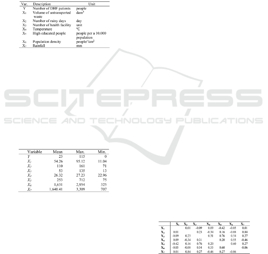
The variables which are suspected of having an

effect on DHF are presented in Figure 3.

Figure 3: Variables assumed to inﬂuence dhf.

4 RESULTS AND DISCUSSION

4.1 Descriptive Analysis

The ﬁrst step in this research is to do a descriptive

analysis that is useful to know the characteristics of

each research variable. Descriptive analysis used in-

cludes average, maximum, and minimum values. The

results of the descriptive analysis are shown in Figure

Figure 4: Descriptive statistics of research variables.

Based on Figure 4, the average number of DHF

patients (Y) in 21 sub-districts of Pasuruan in this

past four years (2015-2018) is 23 people. Lumbang

and Puspo sub-districts have the least number of pa-

tients (none) while Bangil has the highest number of

patients (115 people). The average waste (X

) that

is not transported is 54.26 where Kraton becomes the

sub-district that has the most non-transported waste

reaching up to 95.12 dam

. In contrast, Bangil has

the least non-transported waste which is only 11.04

dam

. The range of maximum and minimum values

of the waste volume that is not transported is very

high. This indicates that the waste services are still

focused on certain sub-districts or in other words, not

comprehensive in all sub-districts. The average num-

ber of rainy days (X

) is 110 where Purwosari has the

most number of rainy days reaching up to 161 days

of rain in a year. Meanwhile, the sub-district with

the least number of rainy days is Gondangwetan and

Winongan, 71 days a year. On the other hand, the av-

erage number of health facilities (X

) is 53. The high-

est number of health facilities is owned by Pandaan

sub-district (135 units) while the least health facili-

ties are owned by Puspo (13 units). The average tem-

perature (X

) is 26.32°C. It is reported that the high-

est temperature occurs in Beji reaching up to 27.23°C

while the lowest temperature is in Purwodadi reach-

ing up to 22.96°C. The average number of educated

population (X

) is 253 where the area with the highest

number of educated people is Bangil (712 people per

a 10,000 population) while the lowest number of edu-

cated people is Lekok (75 people per a 10,000 popu-

lation). The average population density (X

) is 1,631.

The most densely populated area is Pohjentrek with a

population density of 2,954 people/km

whereas the

lowest population density can be found in Lumbang,

only 325 people/km

. The range between the max-

imum and minimum population density is very big.

This means that the population distribution is uneven

or concentrated in certain sub-districts. Last but not

least, the average value of Rainfall (X

) is 1,640.41

where the area with the highest rainfall intensity is

Purwosari reaching up to 3,309 mm in a year. Mean-

while, the area with the lowest rainfall intensity is

Winongan, only 707 mm in a year.

4.2 Multicollinearity Test

Multicollinearity test is applied to see the correla-

tion of each predictor variable used in the regression

model. The existence of perfect multicollinearity can

cause many predictor variables do not have a signiﬁ-

cant effect although the coefﬁcient of determination

is high. To detect multicollinearity, the correlation

coefﬁcient method is used (r). The results of multi-

collinearity test are presented in Figure 5.

Figure 5: Correlation coefﬁcient.

From Table 4, the value of r in each column is

< 0.85 so that all predictor variables are free from

multicollinearity problems.

Data Panel Modelling with Fixed Effect Model (FEM) Approach to Analyze the Inﬂuencing Factors of DHF in Pasuruan Regency

229

4.3 Selection of Panel Data Regression

Model

To choose a model that ﬁts the research data, re-

searchers can conduct the Chow Test, Hausman Test,

and Lagrange Multiplier Test. Chow Test is used to

determine whether or not the differences between the

characteristics of the districts are seen from the inter-

cept on each regression model. From the Chow Test,

it is obtained that F

count

= 5.618 > F

0.05(20;56)

= 1.76

dan p − value = 0.0000 ≤ 0.05 with a level of reli-

ability by 95%. This means that hypothesis H0 re-

jected, there are differences in the regional charac-

teristics presented in the DHF Panel Data regression

equation model of Pasuruan Regency so that the ap-

propriate model must be FEM.

Moreover, the Hausman Test is performed to test

whether or not there is a correlation between the er-

ror component in the model and its predictor vari-

able. The Hausman Test results showed that W

count

79.223 > χ

(005;7)

= 14.07 and p − value = 0.0000 ≤

0.05 with a level of reliability by 95%. It can be said

that the hypothesis H0 is rejected. This points out

that there is no correlation between the error com-

ponent predictor variables on Pasuruan DHF Panel

Data regression equation. Therefore, the correspond-

ing model is FEM.

Because of the two tests above refer FEM as the

appropriate model, it is not necessary to do the La-

grange Multiplier Test.

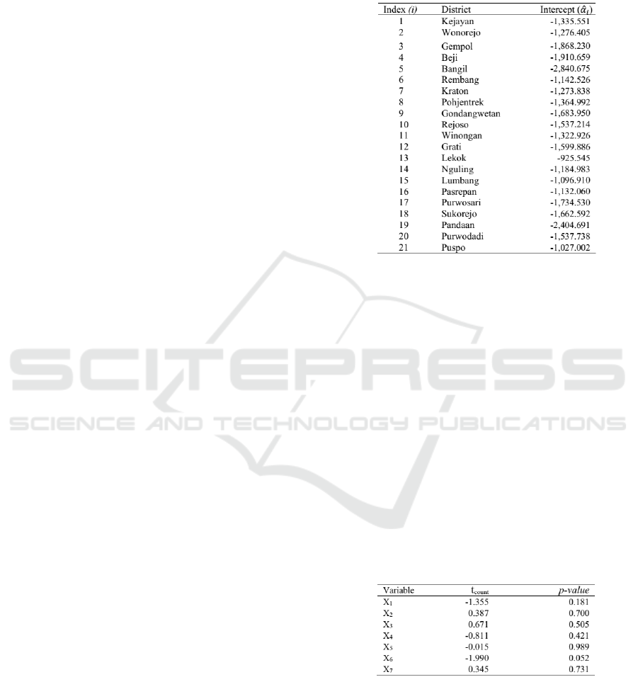
4.4 Model Estimation with FEM

Approach

Here is the estimation of Panel Data regression model

formed by using FEM approach.

α + 1.785X

+ 0.186X

+ 1.470X

+ 32.267X

+ 3.186X

− 0.177X

− 0.014X

(13)

is the intercept that has different values in each

region. This value will distinguish the prediction of

the number of DHF patients in between sub-districts.

Because each region has different characteristics, the

characteristic differences are represented by an inter-

cept variable in the ﬁxed effect Panel Data regression

model. The intercept value for each district is shown

in Figure 6.

Equation 13 shows that the increase in variable Y

is inﬂuenced by the increase in variable X

, X

, and X

. Meanwhile, the increase in variable X

and X

will affect the decrease in variable Y.

Figure 6: Estimated intercept value of each region.

4.5 Classical Assumptions Test

After the estimation of the Panel Data regression

model is obtained, the next step is to carry out the

classical assumption tests which include the Normal-

ity Test, Heteroscedasticity Test, and Autocorrelation

Test.

The Normality Test is done by using the Jarque-

Bera formula. From this test, it is obtained JB =

0.372 < χ

(005;2)

= 5.991 and p − value = 0.83 > 0.05

with a level of reliability by 95%. By that, hypothesis

is accepted meaning that the error is normally dis-

tributed. Then, a Heteroscedasticity Test is performed

to see whether the error variant has a constant nature

or not. Glejser Test is used for the Heteroscedasticity

Test and the values obtained can be seen in Figure 7

below.

Figure 7: Simultaneous test result.

Based on Figure 7, the p-value for each predictor

variable is > 0.05 making the hypothesis H

accepted.

This explains that the error in the model does not con-

tain heteroscedasticity or is constant.

The last classical assumption test is the Autocor-

relation Test that is done by using the Durbin Wat-

son test method. It is obtained that DW = 2.056.

ICASESS 2019 - International Conference on Applied Science, Engineering and Social Science

230

The value is in the area of Hypothesis H

which is

= 1.8291 ≤ DW = 2.101 ≤ 4−d

= 2.1709, mean-

ing that the error in the model is free from the prob-

lem of autocorrelation.

4.6 Signiﬁcance of Parameters Test

After the model has passed all classical assumption

tests, the next step is to do a simultaneous test and par-

tial test to determine the effect of predictor variables

on the response variable both simultaneously and par-

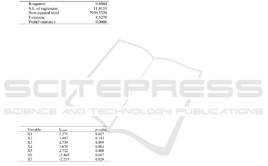
tially. The simultaneous test results are presented in

Figure 8.

Figure 8: Simultaneous test result.

As shown in Figure 8, the value of F

count

8.528 > F

(0.05;27;56)

= 1.686 and p −value = 0.000 <

0.05 and R

= 0.804 with a level of reliability by

95%. This clariﬁes that hypothesis H0 is rejected,

the predictor variable simultaneously affects the re-

sponse variable. The value of R

= 0.804 shows that

the seven predictor variables can affect the number of

DHF patients in Pasuruan by 80.4% while the remain-

ing 19.6% are inﬂuenced by other variables outside

the model.

After that, a partial test is carried out. The results

of the partial test are shown in Figure 9.

Figure 9: Partial test results.

As presented in Figure 9 with a reliability level

of 95%, there are six variables that have a signiﬁcant

effect on the response variable (p − value < 0.05),

namely variable X

, X

, and X

while the

variable X

does not have a signiﬁcant inﬂuence on

the response variable (p − value > 0.05).

5 CONCLUSION AND

SUGGESTION

Based on the results of the analysis, it can be con-

cluded that the Panel Data regression model with

Fixed Effect Model approach can explain the effect of

predictor variables on the response variable. There-

fore, the model equation is:

α + 1.785X

+ 0.186X

+ 1.470X

+ 32.267X

+ 3.186X

− 0.177X

− 0.014X

(14)

From the Equation 14 above, the value of R

0.804 shows that the percentage of all seven predic-

tor variables able to affect the number of DHF pa-

tients in Pasuruan by 80.4% while the other 19.6% are

inﬂuenced by other variables outside this study. Of

the seven predictor variables, there are six variables

that signiﬁcantly inﬂuence the increase in the num-

ber of DHF patients such as waste volume, number of

health facilities, temperature, high-educated popula-

tion, population density, and rainfall.

Last but not least, the Department of Health of Pa-

suruan Regency is suggested to plan the programs and

activities to control and eradicate future DHF by fo-

cusing on the variables that have a signiﬁcant effect

on DHF patients.

In the future the model can be developed into an

application that can be utilized by government or in-

terested organizations.

REFERENCES

Ariani, P. M. (2018). Analisis Faktor yang Berpengaruh

Terhadap Pencegahan Penyakit DBD di Provinsi Jawa

Tengah Menggunakan Regresi Binomial Negatif. Tu-

gas Akhir. Universitas Islam Indonesia, Yogyakarta.

Arsin, A. A. (2013). Epidemiologi demam berdarah dengue

(DBD. Masagena Press, di indonesia.Makassar.

Baltagi, B. H. (2010). Econometric Analysis of Panel Data.

John Wiley & Sons, Ltd, Sussex, 4th edition. west edi-

tion.

Greene, W. (2000). Econometric Analysis. Prentice Hall,

Inc, 4th edition.

Gujarati, D. (2004). Basic Econometrics. The McGraw-Hill

Companies, New York, 4th edition.

Gujarati, D. and P, D. C. (2010). Dasar-dasar Ekonometrika

Edisi 5. Salemba Empat, Jakarta.

Hasirun (2016). Model Spasial Faktor Risiko Kejadian De-

mam Berdarah Dengue di Provinsi Jawa Timur Tahun

2014. Tesis. Universitas Airlangga, Surabaya.

Hsiao, C. (2003). Analysis of Panel Data. Cambridge Uni-

versity Press, New York.

I., A. W., Ratnasari, V., and Wibowo, W. (2017). Analisis

faktor yang berpengaruh terhadap tingkat penganggu-

ran terbuka di provinsi jawa timur menggunakan re-

gresi data panel. Jurnal Sains dan Seni ITS, 6(1).

Kemenkes, R. (2010). Jendela Epidemiologi. Pusat Data

dan Surveilans Epidemiologi Kementerian Kesehatan

Republik Indonesia, Jakarta.

Data Panel Modelling with Fixed Effect Model (FEM) Approach to Analyze the Inﬂuencing Factors of DHF in Pasuruan Regency

231

Kemenkes, R. (2017). Proﬁl Kesehatan Indonesia Tahun

2017. Setjen Kementerian Kesehatan Republik In-

donesia, Jakarta.

Martha, Z. (2015). Pemodelan Regresi Data Panel Pada

Kasus Jumlah Penderita Demam Berdarah Dengue

(DBD) di Kota Bogor.Tesis. Institut Pertanian Bogor,

Bogor.

Rasmanto, M. (2016). Model prediksi kejadian demam

berdarah dengue (dbd) berdasarkan unsur iklim di

kota kendari tahun 2000-2005. Jurnal Ilmiah Maha-

siswa Kesehatan Masyarakat, 1.

Rustiani, N. N. (2017). Pemodelan penyebaran penyakit

demam berdarah dengue (dbd) dengan pendekatan re-

gresi linear berganda. In Prosiding Seminar Nasional

Sainstek 2017. Fakultas MIPA Universitas Udayana.

Sutikno, B., F.k, A., and D, O. (2017). Penerapan regresi

panel data komponen satu arah untuk menentukan

faktor-faktor yang mempengaruhi indeks pembangu-

nan manusia.jurnal matematika integratif unpad.

Widarjono, A. (2013). Ekonometrika Teori dan Aplikasi

Untuk Ekonomi dan Bisnis. Ekonosia FE UII, Yo-

gyakarta.

ICASESS 2019 - International Conference on Applied Science, Engineering and Social Science

232