Prediction and Analysis of the Factors That Influence Volume of Air
Passenger at Banyuwangi Airport using Econometric
Suwander Husada
1
, Endroyono
1
and Yoyon K. Suprapto
1
1
Department of Electrical Engineering, Institute of Institute Teknologi Sepuluh Nopember, Surabaya, Indonesia
Keywords:
Econometric, Passenger Prediction, Airport Masterplan.
Abstract:
The volume of passengers at the airport in the future needs to be predicted. From several air passenger
prediction methods, one of them is the econometric method. This method has the excellence of long-term
predictions and gaining knowledge of economic factors that affect the volume of air passengers. In this study,
several economic factors, such as hotel occupancy, population, rupiah exchange rate, tourism visitor, inflation,
and the Banyuwangi Consumer Price Index (CPI), were analyzed. Pre-analysis data needed before building
the model, including data selection, data description, data pattern recognition, and data completeness. The best
econometric model is obtained from the results of the combination test of each variable. The best econometric
model is used to predict the volume of air passengers in Banyuwangi airport for the next 20 years. From the
results, three factors significantly effect the volume of air passengers, that is, hotel occupancy affect 0.301%,
population affect 0.132%, and the rupiah exchange rate affect -0.481%. To evaluate the accuracy of predictions
using the Mean Absolute Percentage Error (MAPE) with a value of 15,208 %.
1 INTRODUCTION
Indonesia Civil Avition Law No.1 2009, it is stated
that the airport, one of the transportation network
nodes. It encourages and supports industrial and
trade activities. It encourages and supports indus-
trial and trade activities. The economic stability of
Banyuwangi Regency has an impact on the growth of
human and goods mobilization from origin to desti-
nation through air transportation modes. Referring to
the Banyuwangi Airport Master Plan, phase II is es-
timated to serve aircraft passengers around 272,500
passengers per year, but in 2017 volume of air pas-
sengers at Banyuwangi Airport is 188,949 thousand,
and by the end of 2018 air passengers volume is
366,155 people. There is a significant difference be-
tween the master plan projections and existing pas-
senger. Banyuwangi Airport has the potential to ex-
perience density and result in a decrease in the quality
of services for users of air transportation services. In
this condition, there is a high need to evaluate and
projections air volume passengers in the future.
The purpose of this study is to predict the vol-
ume of air passengers for the next 20 years and an-
alyze the factors that effect the volume of passengers
at Banyuwangi Airport. According result of analysis,
it was obtaining knowledge about the factors that in-
fluence the volume of air passengers at Banyuwangi
Airport. The study result can be used as a reference
for policy development.
2 LITERATURE REVIEW
Economic factors affect the volume of passengers at
certain airports, regions or cities. The most com-
mon economic indicators are Gross Domestic Product
(GDP), Per capita GDP, Population (Pop), Income,
and Per Capita Income (Guo and Zhong, 2017). There
are many studies that discuss the relationship between
air passenger volume and economic variables.
Husada, S., Endroyono, . and Suprapto, Y.
Prediction and Analysis of the Factors That Influence Volume of Air Passenger at Banyuwangi Airport using Econometric.
DOI: 10.5220/0009880301730179
In Proceedings of the 2nd International Conference on Applied Science, Engineering and Social Sciences (ICASESS 2019), pages 173-179
ISBN: 978-989-758-452-7
Copyright
c
 2020 by SCITEPRESS – Science and Technology Publications, Lda. All rights reserved
173

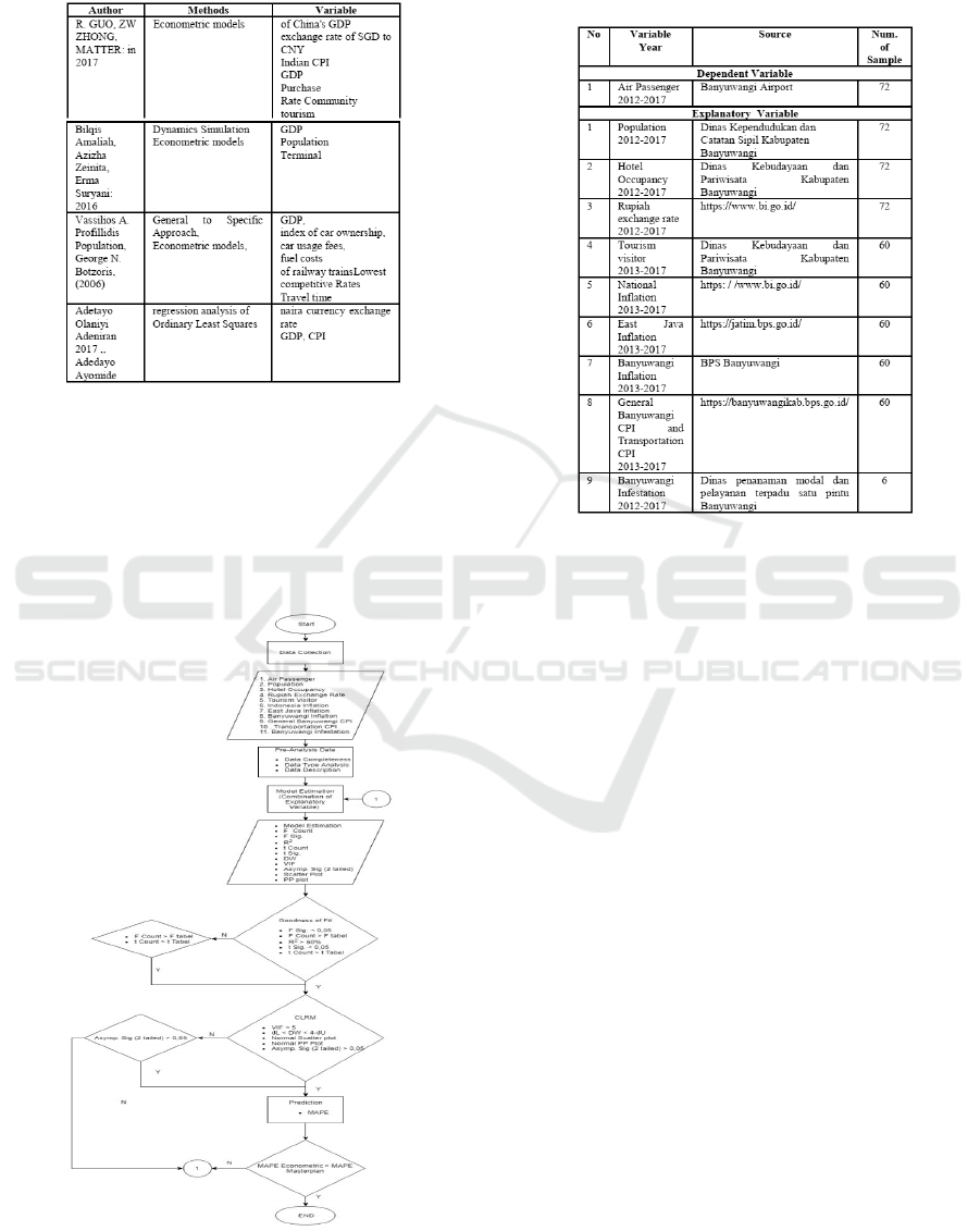
Figure 1. Provides insight into several economic
indicators that have been used to estimate the volume
of air passenger.
Figure 1: Literature Review.
3 METHODOLOGY
To solve the problem, the process is carried out refer-
ring to the methodology illustrated in Figure 2.
Figure 2: Methodology flow chart
3.1 Data Collection
Data in this study was collected from agencies, and
website agencies, as shown in Figure 3.
Figure 3: Dependent Variable and Explanatory Variable.
3.2 Pre-analysis Data
Pre-analysis of data consists of :
3.2.1 Data Completeness
Completeness of data includes independent variables,
explanatory variables, number of data, and year,
shown in Figure 3.
3.2.2 Data Type Analysis
Data type in this research:
• Data Type : Quantitative data
• Data Classified : secondary data
• Measurement : Interval – Ratio
3.2.3 Description of Data Graphically
To simplify data analysis, detect trends, seasonal and
data patterns, the data is presented using a line chart
graph, where the X axis for time (month), and the
Yaxis for volume.
ICASESS 2019 - International Conference on Applied Science, Engineering and Social Science
174

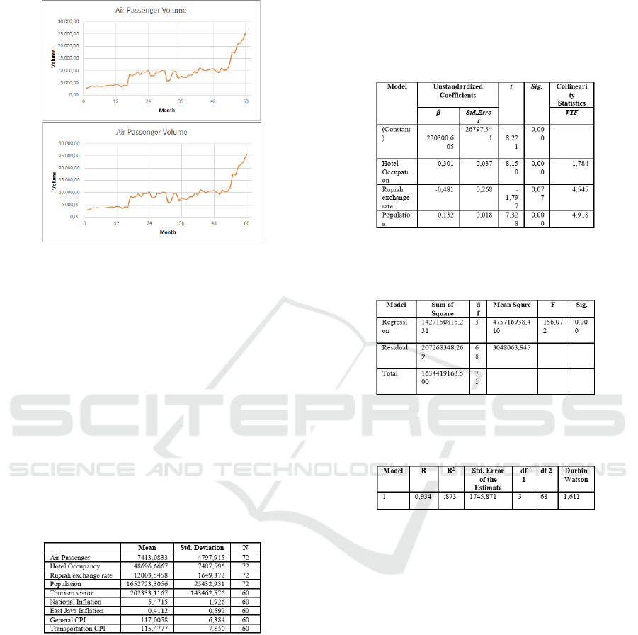
Example of graphically shown in Figure 4.
Figure 4: Description of data graphically
There are several data that have the potential to be
included in the model, comprise:
• Investment data of Banyuwangi in 2012-2017, the
data has annual intervals so that it requires inter-
polation of monthly intervals. And it is feared that
it will cause inaccuracies in the model.
• Banyuwangi Inflation, there are similarities be-
tween Banyuwangi inflation data and East Java in-
flation, In this study used East Java inflation.
3.2.4 Data Description Numerically
Data description numerically is shown in Figure 5.
to get the mean, standard deviation, and Number of
Sample (N).
Figure 5: Descriptive Statistic Table.
3.3 Model Estimation
Regression analysis, implemented in equation (1), is
needed to measure the strength and direction of pas-
senger relationships and explanatory variables. To de-
termine constants, using the Ordinary Least Squares
(OLS) method. In linear regression analysis with
OLS, it is necessary to pass the test of the classical
linear regression model (CLRM).
Y = β
0
+ β
1
x
1
+ β
2
x
2
+ ... + β
n
x
n
(1)
Y = Dependent Variable β
0
= Constants β
1
, β
2
...β
n
= Estimated regression coefficient x
1
, x
2
, . . . x
n
=
Explanatory Variable
Coefficients table is shown in Figure 6 produces
values of : β
0
, β
1
, β
2
...β
n
, t count, t Sig., Variance
Inflation Factor (VIF) value.
Figure 6: Coefficients table.
Anova table is shown Figure 7 produces values of
: Degree of Freedom (df), F count, and F Sig
Figure 7: Anova Table.
Model Summary is sown in Figure 8 .produces
values of: R , R2 , Durbin Watson (DW)
Figure 8: Model Summary Table.
3.4 Goodness of Fit / Model Feasibility
Test
The accuracy of the regression model obtained in esti-
mating the actual value can be measured by a simulta-
neous regression coefficient test (F-Test), coefficient
of determination (R2), and test individual coefficients
test (t-Test).
3.4.1 F-test
The F-test is used to determine whether the Explana-
tory variable X
1
, x
2
,...x
n
has a significant influence on
the dependent variable Y simultaneously.
• Compare the F Sig to significance level
– if value of F Sig. < 0.05, explanatory variables
have a significant effect simultaneously on de-
pendent variable.
Prediction and Analysis of the Factors That Influence Volume of Air Passenger at Banyuwangi Airport using Econometric
175

– if value of F Sig. > 0.05, explanatory variables
have no significant effect simultaneously on de-
pendent variable, or compare F count to t table
value.
• Compare t count to t table value
– if F count > F table value, Explanatory vari-
ables have a significant effect simultaneously
on dependent variable.
– if F count < F table value, Explanatory vari-
ables have no significant effect simultaneously
on dependent variable.
3.4.2 Coefficient of Determination (R
2
)
Coefficient of Determination using to measure how
far the ability of the model explains the dependent
variable (Kuncoro, 2001). Implemented in the equa-
tion (2).
Coe f ficiento f Determination = (R)
2
.100% (2)
3.4.3 Individual Coefficients Test (t-Test)
The t-test is used to find out how far the explanatory
variables effect the dependent variables individually
(Kuncoro, 2001) If t Sig. < Significance level (α),
the model estimation is declared feasible (Kuncoro,
2001).
• Compare the t Sig to significance level (Siregar,
2013).
– if value of t Sig. < 0.05, explanatory variables
have a significant effect individually on depen-
dent variable.
– if the value of t Sig. > 0.05, explanatory vari-
ables have no significant effect individually on
dependent variable. or Compare t count and t
table value.
• Compare t count to t Table value (Siregar, 2013).
– if t count ≥ t table value, explanatory variables
have a significant effect individually on depen-
dent variable.
– If -t table value ≤ t count ≤ t table value ex-
planatory variables have a significant effect in-
dividually on dependent variable.
3.5 Classical Linear Regression Models
(CLRM)
The model must pass the CLRM, comprise:
3.5.1 Multicollinearity
Multicollinearity is a state of high intercorrelations
among the explanatory variables. The model is de-
clared free from multicollinearity if the VIF value <
5 . Using VIF value.
• if VIF value < 5, there are no symptoms of Mul-
ticollinearity.
• if VIF value > 5, there are symptoms of Multi-
collinearity.
3.5.2 Autocorrelation / Independence of
Observations
In time series data, autocorrelation is defined the er-
ror for one time period t is correlated with the error
for a subsequent time period t-1. To measure of auto-
correlation uses durbin watson test. Compare the DW
value with the value of dL and dU on the DW table
level. The value of dL and dU are shown in Figure 9.
1. dU < DW< 4-dU item If DW value fall in incon-
clusive area, uses Run test to measure of autocor-
relation (Profillidis and Botzoris, 2006) Figure 10.
Figure 9: DW Table Level.
T : Number of samples K : Number of variables
dL: Lower limit of Durbin Watson dU: Upper limit of
Durbin Watson
Figure 10: Description of Autocorrelation Using DW
3.5.3 Run Test
Run test is an alternative test to test the autocorrela-
tion if the DW value fall in conculsion area. The test
applied by run the randomization test (Profillidis and
Botzoris, 2006). Decision in run test, if Asymp. Sig.
(2-tailed) > 0,05 , there are no symptoms of autocor-
relation.
3.5.4 Heteroscedasticity
The Heteroscedasticity test is a test that assesses
whether there is an inequality of variance from the
residual for all observations in the linear regression
model (Kuncoro, 2001). Heteroscedasticity test ana-
lyzes the Scatter plot. The Scatter Plot Graph as seen
ICASESS 2019 - International Conference on Applied Science, Engineering and Social Science
176

as Figure 11 created with y and x axis,where x axis
is Studentized Residual (SRESID) and y axis is Stan-
dardized Predicted Value (ZPRED)”.
Figure 11: A There are symptoms of heteroskedasticity, B
No Symptoms of Heteroskedasticity
3.5.5 Normality
The results of the normality test by observing the dis-
tribution of Probability Plots (PP Plots). If the distri-
bution of these points approaches or is in a straight
line (diagonal), then it is said that (residual data) is
normally distributed, but if the distribution of these
points is far from the line, then the skewed distribu-
tion as seen as Figure 12.
Figure 12: A PP plot with skewed distribution, B Normal
PP Plot
3.6 Predictions
Prediction is the process of systematically estimating
something that is most likely to occur in the future
based on past and present information.
• Winter additive exponential methode Three com-
ponents winter additive exponential smoothing
implemented in equation (3), (4), (5), and (6) (In,
2017):
1. Prediction
Y
t+m
= S
t
+ mb
t
+ l
t−L+m
(3)
2. Overall Smoothing
S
t
= a(X
t
− l
t−1
) + (1 − a)(S
t
+ b
t−1
) (4)
3. Smoothing trend
b
t
= β(S
t
− S
t−1
) + (1 − β)b
t
− 1 (5)
4. Seasonal Refinement
l
t
= Y (X
t
− S
t
) + (1 −Y )l
t−1
(6)
Where :
S
t
= Smoothing value for t period.
X
t
= Actual value in the final period t
b
t
= Value of trend smoothing
α = Smoothing parameters for data (0 < α <1)
Y = Seasonal smoothing parameters (0 < y <1)
β = Smoothing parameters for trends (0< β <1)
l
t
= Seasonal adjustment factors
L = Seasonal length
Y
t
+ m = Forcasting for m periode from t
m = Number of periods to forecast
3.7 Evaluation of Predictions
The prediction model is validated using Mean Abso-
lute Percentage Error (MAPE) (7).
MAPE =
Σ
|ei|
X
i
100
%
n
=
Σ
|X
i
−F
i
|
X
i
100
%
n
(7)
4 RESULTS AND DISCUSSION
From the regression analysis procedure performed,
three estimations of the econometric model were
built. Each model results from a combination of ex-
planatory variables.
4.1 Model 1
Model 1 is built using eight explanatory variables,
with 95% Significance level (α), and number of sam-
ples (N) 60, the details as shown in Figure 13.
Refer to Figure 13, the R2 = 85,9%, meaning the
explanatory variable can explain the dependent vari-
ables well and has a strong relationship. Explanatory
variables have a significant effect simultaneously on
dependent variable referring to F.Sig. (0,000) < Sig-
nificance level (0,05). t Sig of x1, x2, x3 and , x4 <
0,05 it means they have a significant effect individu-
ally on dependent variabel. t Sig. of x5, x6, x7 and ,
x8 > t Significance level, so it need to compare t count
to t table. t count of x5, x6, x7 and , x8 < 1,675. It
declare , the explanatory variables have no significant
effect individually on dependent variable.
Prediction and Analysis of the Factors That Influence Volume of Air Passenger at Banyuwangi Airport using Econometric
177

According the result of t-test, model 1 not pass
feasibility test.
Figure 13: Model 1 Information Table
4.2 Model 2
Model 2 is Built with four explanatory variables, with
95%Significance level (α), and number of sample (N)
60, the details as shown in Figure 14 .
Figure 14: Model 2 Information Table
Refer to Figure 14, the R2 = 84,7%, meaning the
explanatory variable can explain the dependent vari-
ables well and has a strong relationship. Explanatory
variables have a significant effect simultaneously on
dependent variable referring to F.Sig. (0,000) < Sig-
nificance level (0,05). t Sig of x1, x3and ,x4 < 0,05
it means they have a significant effect individually on
dependent, but t Sig of x3> Significance level, so it
need to compare t count to t table. t count of x3(7.213)
> 1.674. It declare all explanatory variables have
significant effect individually on dependent variable.
Model 2 pass the Multicollinearity test. According
to all VIF value < 5. For autocorrelation test, DW
value < dL, it means model 2 have a positive autocor-
relation. According the result of autocorrelation test,
model 2 not pass CLRM test.
4.3 Model 3
Model 3 was Built with three explanatory variables,
with 95% Significance level (α), and number of sam-
ple (N) 72, the details as shown in Figure 15.
Figure 15: Model 3 Information Table
Refer to Figure 8, the R2 = 87,3, meaning the ex-
planatory can explain the dependent variables well
and has a strong relationship. Explanatory variables
have a significant effect simultaneously on dependent
variable referring to F.Sig. (0,000) < Significance
level (0,05). t Sig. of x1,and x2 < 0,05 it means
they have a significant effect individually on depen-
dent, but t Sig. of x3> t Significance level, so it need
to compare t count to t table. t count of x3(-1.797)
< - 1.670. It declare all explanatory variables have
significant effect individually on dependent variable.
Model 3 pass the Multicollinearity test according to
all VIF value < 5. For autocorrelation test, DW value
< dU, DW value fall in inconclusive area, to solved
this condition we uses a Run test. Result of Run test
as shown in Figure 16.
Refer to Figure 16, value of Asymp. Sig(2-tailed)
0,476 > 0,05, it means model 3 no autocorrelation.
From Figure 12 shows that the point distribution does
not form a particular pattern / path, so it can be con-
cluded no heteroscedasticity. Distribution of points
from Figure 17 normal P-P Plot.
ICASESS 2019 - International Conference on Applied Science, Engineering and Social Science
178

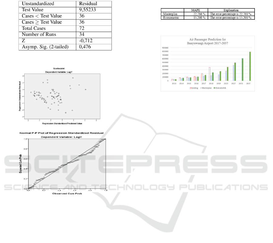
The above plot is relatively close to a straight line,
so it can be concluded that the data residuals are dis-
tributed normally.
Figure 16: Run test result.
Figure 17: PP Plot
4.4 Predictions for the Next 20 Years
After getting the model, we predict each explanatory
variable. From the observations of the data on each
variable, with the presence of seasonal trends and pat-
terns, the use of predictions suitable for each variable
is as follows:
1. Population Winter Additives
2. Hotel Occupancy Winter Additives
3. Currency Exchange Winter Additives
Based on the econometric model 3, the volume of
air passengers in Banyuwangi is predicted for the next
20 years. Predictions from 2017 to 2037. Prediction
results are shown in Figure 19.
4.5 Prediction Validation
Figure 18 shows comparation MAPE value for econo-
metric prediction and Masterplan prediction.
Figure 18: Comparation MAPE Value.
Figure 19: Results of model econometric predictions
5 CONCLUSIONS
The results of the analysis; the variables that sig-
nificantly influence the volume of air passengers at
Banyuwangi airport are Hotels Occupancy, Rupiah
exchange rates, and Population, with coefficients of
value 0, 301, -0.481, and 0.132. A negative sign
on the rupiah exchange rate shows an inverse rela-
tionship. With the MAPE value of 15,208 %, the
prediction of passengers at Banyuwangi Airport us-
ing econometrics is declared feasible. Therefore,
it is concluded that the economic model provides
a good estimate of the volume of air passengers at
Banyuwangi Airport.
REFERENCES
Guo, R. and Zhong, Z. W. (2017). Forecasting air passen-
ger volume in singapore: determining the explanatory
variables for econometric models. MATTER: Interna-
tional Journal of Science and Technology, 3(1).
In, H. (2017). Pemulusan eksponensial dengan metode holt
winter additive damped. UNHAS Repository.
Kuncoro, M. (2001). Metodde kuantitatif, teori dan aplikasi
untuk bisnis dan ekonomi, upp amp ykpn.
Profillidis, V. A. and Botzoris, G. N. (2006). Economet-
ric models for the forecast of passenger demand in
greece. Journal of Statistics and Management Sys-
tems, 9(1):37–54.
Siregar, S. (2013). Metode penelitian kuantitatif spss. Yo-
gyakarta: Prenada Media Group.
Prediction and Analysis of the Factors That Influence Volume of Air Passenger at Banyuwangi Airport using Econometric
179