Machine Learning System for Rainfall Estimates from Single

Polarization Radar

Tinar Pamuji Waskita

1,2

, Adhi Harmoko Saputro

Ardhasena Sopaheluwakan

and Muhammad

Ryan

Department of Physics, Faculty of Mathematics and Sciences, Universitas Indonesia, Depok 16424, Indonesia

Agency for Meteorology, Climatology and Geophysics, Jakarta 10720, Indonesia

Keywords: rainfall, radar, machine learning, multi layer perceptron

Abstract: Rainfall becomes one of the weather parameters that is most widely considered because the phenomenon of

its occurrence can significantly affect human activities, including in agriculture, plantations, fisheries,

transportation and others. In addition, rainfall information is very important to do weather analysis, especially

in analyzing the occurrence of floods caused by heavy rains so there is a need for accurate rainfall information.

This study aims to obtain an optimal rainfall estimation system at locations where there is no direct rainfall

observation data. Machine learning is one branch of artificial intelligence that provides a learning system for

machines to learn automatically without explicit instruction. The machine learning used in this study is Multi

layer perceptron (MLP), with backpropagation as a gradient value search algorithm and adam optimizer as an

optimization function. The structure of the MLP used is 2 hidden layers which in the first hidden layer uses 7

neurons with a hyperbolic tangent activation function and the second hidden layer contains 3 neurons and the

activation function is sigmoid and finally the output layer, the activation function used is pure linear. MLP

system input data is radar data, reflectivity, radial velocity, spectrum width and radar rain estimation data

which are validated with automatic rain observation data around the Single Polarization Radar observation in

Yogyakarta. The results using MLP can improve rain detection accuracy by 79% and reduce the error value

in the estimated rainfall.

1 INTRODUCTION

Indonesia is a humid archipelago and equatorial

monsoon region (Tjasyono, B.H.K., and Harijono,

S.W.B, 2007), many hydrometeorological natural

disasters occur throughout the year, including

Yogyakarta. Hydrometeorological disasters are

disasters related to changes in the normal water cycle,

such as flash floods (Minervino, A.C and Duarte, E.C,

2015). Hydrometeorological disasters in the current

period show an increasing trend (Adi S. , 2013).

Hydrometeorological disasters can seriously damage

infrastructure, significant economic losses and often

loss of life (Paul, S.H., Sharif, H.O., and Crawford,

A.M.G, 2018). Rainfall is precipitate in liquid form

which is largely a direct result of the condensation of

water droplets in the clouds, followed by growth to a

size large enough to overcome the effect of air

buoyancy forces (Tjasyono, B.H.K., and Harijono,

S.W.B, 2007) .

Single polarization radar is a remote sensing

technology that can be used to determine the

distribution of rain in locations where there is no

rainfall measurement tool. A single polarization radar

measures rainfall in real-time and provides high-

resolution data for short-term rainfall forecasts, also

known as nowcasting (Codo, M., and Rico-Ramirez,

M.A., 2018). Radar emits electromagnetic waves at

the frequency of microwaves in the form of pulses

into the atmosphere through the transmitter. When a

pulse hits an object, the electromagnetic wave is

partly returned to the weather radar which is received

as reflected energy called reflectivity. The amount of

reflectivity depends on the physical parameters of the

object.

Radar transmits microwaves and receives

backscattering radiation from precipitation particles

through radar reflectivity (Z), which is related to

rainfall rate (R) using a semi-empirical equation of

the form Z = a𝑅



(Germann, U., Galli, G. Boscacci,

M., and Bolliger, M., 2006). However, parameters a

Pamuji Waskita, T., Harmoko Saputro, A., Sopaheluwakan, A. and Ryan, M.

Machine Learning System for Rainfall Estimates from Single Polarization Radar.

DOI: 10.5220/0009409400410048

In Proceedings of the International Conferences on Information System and Technology (CONRIST 2019), pages 41-48

ISBN: 978-989-758-453-4

and b of the Z-R relation equation are known to

depend on rainfall type and rainfall size distribution.

The use of the constant Z-R relation equation

contributes to errors in the estimation of radar rainfall

(Harrison,D.L., Driscoll,S.J., and Kitchen,M , 2000).

Radar has limitations that cause errors in

estimating rain and rain forecasts by nowcasting,

when the distance from the radar increases, naturally

there is also an increase in the volume of radar

sampling (Rico-Ramirez, M.A., and Cluckie, I.D,

2007). At higher altitudes, the distribution of the

hydrometeor changes, causing a difference between

the measured rainfall and the rainfall that actually

falls to the ground, so it is necessary to determine the

right technique for estimating using radar. The Single

Polarization Radar in Yogyakarta is a Baron branded

C-Band radar, which has a frequency of 5.2-5.9 GHz

and a wavelength of 5-5.7 cm and Radar Yogyakarta

began operations in 2016. In this research, a statistical

/ engineering based approach is used to improve the

estimation of rainfall in Yogyakarta's Single

Polarization Radar using VCP 21 with 9 elevations.

There are two classifications of rain estimation

techniques using radar, namely: Physical-based

techniques and statistical / engineering-based

techniques (Bringi, V. N. and Chandrasekar, V,

2001). Physically based techniques are used to find

the relationship between the observation radar and

precipitation levels of observation, such as the use of

relational equation Z-R precise in determining the

estimated rainfall while using statistical techniques

such as machine learning algorithms.

Machine learning is an application of artificial

intelligence (AI) that provides a system of ability to

learn automatically and improve from experience

without being completely programmed

(Chandrasekar, V., Tan, H., and Chen, H.,

2017)(Chandrasekar, Tan, and Chen, 2017). Machine

learning spends on developing computer programs

that can be accessed and used for self-study. The

machine learning used in this study is a multi-layer

perceptron (MLP), with backpropagation as a

gradient value search algorithm and adam optimizer

as an optimization function. The structure of the MLP

used is 2 hidden layers which in the first hidden layer

uses 5 neurons with a hyperbolic tanget activation

function and the second hidden layer contains 3

neurons and the activation function is sigmoid and

finally the output layer, the activation function used

is pure linear. MLP system input data is radar data,

reflectivity, radial velocity, spectrum width and radar

rain estimation data which are validated with

automatic rain observation data around the Single

Polarization Radar observation in Yogyakarta.

At the training stage of machine learning network

will produce the best network and the best network

will be tested with new radar data then verified. The

results of the verification value will show and

improve the rainfall estimation model using a single

polarization radar around the study area. An optimal

rainfall estimation system will further benefit weather

forecasters in providing early warning information

for heavy rainfall and in providing extreme weather

analysis at locations where there is no direct rainfall

observation.

2 STUDY AREAS AND DATASET

This study, the results of three radar data outputs are

reflectivity, radial velocity, and width spectrum and

the results of radar rain estimation using the Marshall-

Palmer Z-R relation, will be used as input for MLP.

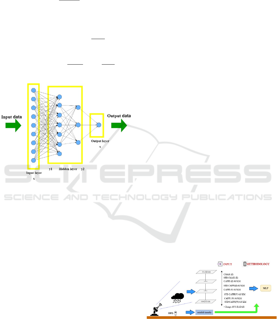
The reflectivity data used are the CMAX(Z) product

reflectivity, the CMAX(Z) product reflectivity

deviation standard, the CAPPI(Z) product reflectivity

0.5 km and the CAPPI(Z) product deviation

reflectivity standard 0.5 km. For radial velocity and

spectrum width data used from CAPPI (V) 0.5 km

and CAPPI (W) 0.5 km. The use of CAPPI 0.5 km

product on reflectivity data, radial velocity data, and

width spectrum data due to the closest surface, for

CMAX products (taking maximum value) on the

reflectivity value can represent conditions vertically

at an altitude of 0.5-30 km (Ali, A and Hidayati,S,

2016). In addition, the distance between automatic

rainfall data and radar is included as additional input.

Furthermore, the 10 inputs are processed using MLP

and automatic rain observation data from an

automated weather station (AWS) will be used as a

target / model validation.

Observation rainfall data used as a comparison of

MLP is AWS data for 2017-2018 in 4 locations,

namely Kulon Progo, Gajah Mada University, Bantul

and Sleman. Data of Automatic rainfall observers is

accumulated per hour. The following is the

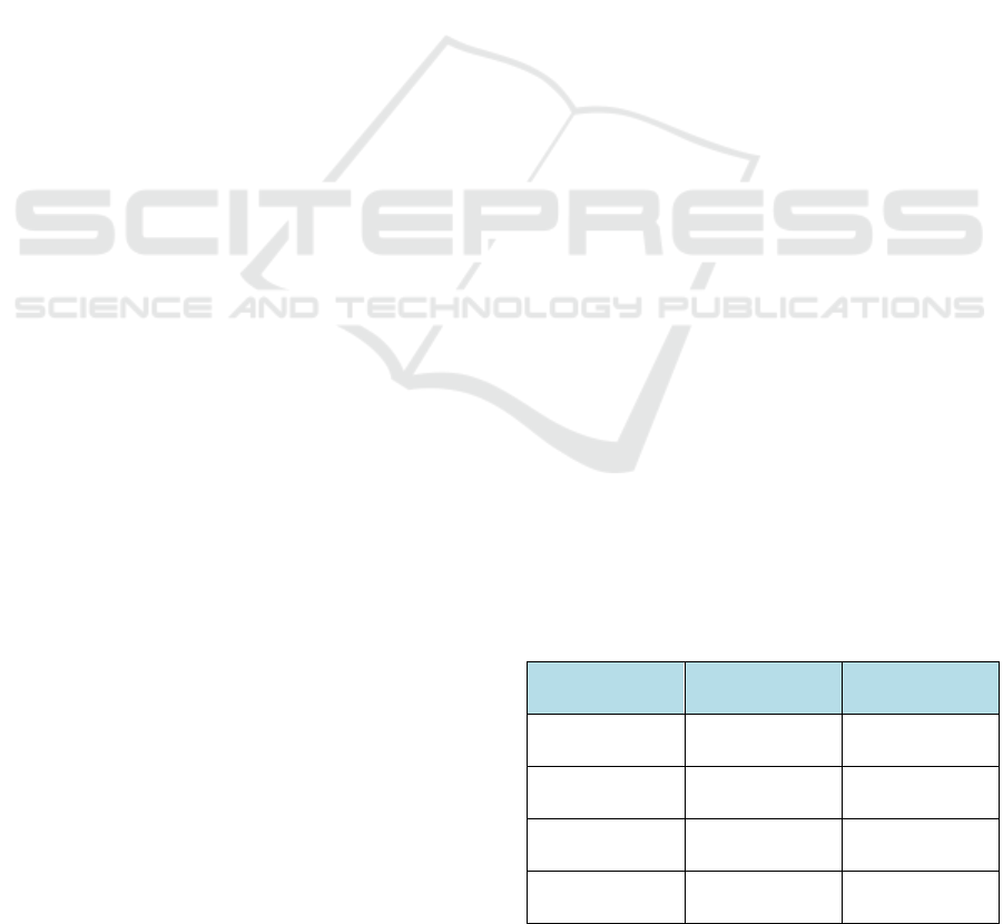
availability of AWS data shown in table 1.

Table 1. Automatic rainfall observation data used

Location Coordinate Total data

(mm/hours)

Kulon-Progo -7,890242;

110,100552

1342

Sleman -7,75016;

110,419759

550

Bantul -7,90736;

110,365048

3163

Gajah Mada

Universit

-7,7704589;

110,3798372

3111

CONRIST 2019 - International Conferences on Information System and Technology

Radar data is processed using python with 2 (two)

stages, namely the data extracting stage and the

training model stage. Data extracting stage is the

stage where the radar data value at the point of

observation of rainfall is automatically extracted.

After the radar product is extracted, the radar value is

used as a predictor while the observed rainfall value

is made a predictor in the MLP model.

The training stage of machine learning network

will produce the best network and the best network

will be tested with new radar data then verified. So

the results of the verification value will show and

improve the rainfall estimation model using a single

polarization radar around the study area. An optimal

rainfall estimation system will further benefit weather

forecasters in providing early warning information

for heavy rainfall and in providing extreme weather

analysis at locations where there is no direct rainfall

observation.

3 RESEARCH METHODOLOGY

3.1 Radar

A single polarization radar has three types of data

output namely reflectivity, radial velocity and

spectral width (Raghavan, 2003). Reflectivity (Z)

states the amount of energy reflectivity returning

from an object, depending on the size, shape and

composition of the object. The amount of energy

received by the radar is much smaller than the energy

that was transmitted at the beginning. The following

radar equation describes the calculation of the amount

of energy returned by the radar, which is very

dependent on the magnitude of the Power Transmit

and the type of radar band used, the greater the object

and the energy received, the greater the reflectivity

value.

𝑃𝑟 









 













𝐾











(1)

Description:

Pr: average power of radio waves returned to radar

(watts)

Pt: Peak wave power emitted by radar (watts)

G: Antenna gain

H: length of radar pulses in the air (m)

θΦ: radi wave width in vertical and horizontal

(radians)

λ: wavelength emitted (m)

𝐾



: refractive index

r: distance from the radar to the target (m)

Z: Radar reflectivity factor (mm

)

The first term of the equation above illustrates the

geometrical composition which will be represented

by the velocity of the electromagnetic waves which

refers to the velocity of light propagation. The second

term of the equation is about the parameters of the

radar system, consisting of the type of polarization

(horizontal and or vertical), antenna gain and

wavelength, the amount of power transmitter and the

amount of pulse used in operations. The resulting data

resolution will be greatly influenced by the choice of

sampling parameters, antenna speed and Pulse

Frequency Repetition used which all depend on the

radar system technical specifications. And the third

term depends on the distance and characteristics of

the target. The radar parameters are relatively fixed,

and if the transmitter is operated and used with a

constant output arrangement, the equation can be

simplified to:

𝑃𝑟 











𝑍 (2)

Where C is a radar constant. The value of Z can be

calculated by the equation:

𝑍

∑

𝐷







(3)

Z values vary between 0.001 and 10,000,000, to make

it easier to understand, use a decibel scale:

𝑍



𝑑𝐵𝑍



10 𝑙𝑜𝑔





𝑍



(4)

dBZ=10𝑙𝑜𝑔



 







 







(5)

The value of Z is proportional to the sum of the entire

particle diameter raised to six in a sample volume,

because the size of the drops is usually measured in

millimeters (mm), and the volume is usually

expressed in units of cubic meters (m

), so Z has a

unit of mm

For the purposes of hydrology connecting signal

strength with observed rainfall, an equation that

combines radar reflectivity and rainfall is needed.

This equation is the approach and empirical

relationship between Z and R. The relationship

between Z and R is drawn in exponential form, as

follows:

𝑍𝑎𝑅



(6)

Where a and b are positive empirical constants whose

value depends on the geographical location and

climate conditions / type of rain. The coefficient a

represents the condition for the median diameter of

the drop size in a sample volume. The greater the

value of a, the median size of drops in a sample

volume indicates a larger diameter. While the

coefficient b represents the equilibrium condition

changes in the size of the drops. The results of rain

estimation using the Marshall-Palmer Z-R relation is

Machine Learning System for Rainfall Estimates from Single Polarization Radar

used to master regional variability in the distribution

of raindrop sizes in Indonesia (M. Marzuki, H.

Hashiguchi, M. K. Yamamoto2, S. Mori and M. D.

Yamanaka, 2013).

Radar transmits electromagnetic waves using

units of power transmit and operational frequency.

Changes in frequency from higher droplets will be

processed and recognized as movements approaching

the radar, while changes in frequency from lower

echo replies are recognized as echos moving away

from the radar. Radar routinely measures speed and is

used to detect wind speeds, tornadoes, and hurricanes.

This echo movement data is called radial velocity (V)

data. Velocity radial data can be used as a validation

medium for echo reflectivity / intensity for the

forecaster to recognize meteorological and non-

meteorological echoes, because generally rain

patterns have different patterns from other echoes.

And especially for Ground Clutter echo has a zero

radial speed value. V data not only describes the

movement of rain particles, but Velocity data is very

helpful in describing phenomena in two scales,

namely the large scale (largescale) and small scale

(mesoscale). Large scale (largescale) describes

phenomena that occur in all regions and potential

SHEAR that supports rotation while small scale

(mesoscale) describes whether Converging,

Divergent or rotating winds are also used to diagnose

Couplets (two adjacent Inbound and outbound areas

to detect Convergence , Divergence or rotation).

The spectral width (W) data produced by the

weather radar is taken from processing the frequency

signal reflected by the object and received by the

weather radar. In one sampling volume each droplet

has a different speed and direction of motion, the

value of the deviation of each droplet is displayed by

the spectral width data. Information obtained from the

value of W in the form of air lability. A small width

value indicates that in the sampling volume there is

no difference in speed (stable) and a large width value

indicates there is a difference in the speed of the

hydrometeor in the sampling volume (unstable). W

value gives information about the possibility of

windshear, turbulence, mesocyclone.

Constant altitude plan position indicator (CAPPI)

is a radar product that is made based on the height

input desired by the user. The height referred to in this

product is the height of the MSL. It is recommended

to apply the Pseudo-CAPPI algorithm to maximize its

output, the height of this cappi product has the same

value both near and far from the radar. The CAPPI

algorithm will only display data available at the

desired height at each elevation available. When there

is no data at the desired height then the data is blank.

The Maximum Reflectivity (CMAX) product

represents the maximum reflectivity value between

two heights for each cell of volume. In other words,

able to show the maximum detectable reflectivity of

each pixel between the selected user height, including

the East-West and North-South profiles from the

maximum in the side panel. This product was

produced based on a volume scan. A minimum and

maximum height set by the user and defaults to 0.5

and 30 kilometers. The advantages of MAX products

include being able to display peaks and side views in

the same window so as to give a three-dimensional

(3D) impression of the weather situation. In addition,

ground clutter will be reduced when choosing a

bottom height that is higher than the radar installation

height. However, this product is less useful for data

speeds because only absolute speeds are displayed.

The product is very useful especially for reflectivity

data analysis to medium distances.

3.2 Multi Layer Perceptron (MLP)

MLP structure consists of input layer, hidden

layer and output layer. The back-propagation

algorithm is the most popular approach, which not

only overcomes the weaknesses of the large network

generated in the previous section, but also makes this

network a powerful tool for a number of other

applications, beyond pattern recognition

(Theodoridis, S., Koutroumbas, K., Koutroumbas, K.,

& Koutroumbas, K. , 2008). This approach is usually

to improve architecture and calculate synaptic

parameters so as to minimize the appropriate cost

function of the output. However, such an approach is

a difficulty in the discontinuity of the step function

(activation), promoting differentiation with respect to

unknown parameters. Synaptic weight The

perceptron multilayer architecture has so far been

developed by Nouron McCulloch-Pitts (Theodoridis,

S., Koutroumbas, K., Koutroumbas, K., &

Koutroumbas, K. , 2008). The most complex task to

implement the hardware artificial neural networks is

the non-linear activation function. Common

examples of activation function include hard-limiter,

saturated linear, hyperbolic tangent function and

sigmoid function (A. Armoto, L. Fanucci, E.P.

Scilingo and D.De Rossi, 2011).

The most common non-linear activation

functions, which are used in the artificial neural

networks, are the sigmoid function and the

hyperbolic, these functions are mainly used in

statistics, bio-mathematics, physics, engineering,

economic science, etc tangent (A. Armoto, L.

CONRIST 2019 - International Conferences on Information System and Technology

Fanucci, E.P. Scilingo and D.De Rossi, 2011). The

general equation is as follows:

𝑦







𝑑 (7)

where a, b, c and d are constants.

The sigmoid function is a particular case of Eq.

(7) where we put a = 1, b = 1, c = 0 and d = 0. The

equation thus becoming:

𝑦𝑆



𝑥











(8)

On the other hand, when a = 2, b = 2, c = 0 and d

= 1, the equation represents the hyperbolic tangent:

𝑦𝑇



𝑥











1













(9)

The following is a picture of MLP network

architecture in this study:

Figure 1. MLP network architecture

Adaptive Moment Estimation (Adam) is a very

popular training algorithm for deep neural networks,

implemented in many machine learning frameworks

(Bock & Weis, 2019). Adaptive optimization

algorithms, such as Adam and have proven better

optimization performance than stochastic gradient

descent (SGD) in several scenarios (Zhang, 2019).

According to Kingma & Ba (2015), the Adam

algorithm is a method that is easy to implement,

computationally efficient, has few memory

requirements, is not volatile for scaling gradients

diagonally, and is suitable for large problems in terms

of data and / or parameters. This method is also

suitable for purposes and problems that are not

stationary with gradients that have a lot of noise and

data that are not continuous.

In this study, MLP used has 2 (two) hidden layers,

which in the first and second hidden layers have

different activation functions. The first hidden layer

uses the sigmoid activation function and the second

hidden layer uses the tangent activation function, with

backpropagation as the gradient value finder

algorithm and Adam optimizer as the optimization

function. The structure of the MLP used 9 inputs, 2

hidden layers which in the first hidden layer uses 7

neurons with a hyperbolic tanget activation function

and the second hidden layer contains 3 neurons and

the activation function is sigmoid and finally the

output layer, the activation function used is pure

linear

The results of rainfall estimation using the

Marshall-Palmer Z-R relation is used to master

regional variability in the distribution of raindrop

sizes in Indonesia (M. Marzuki, H. Hashiguchi, M. K.

Yamamoto2, S. Mori and M. D. Yamanaka, 2013).

CAPPI (V) 0.5 km products and CAPPI (W) 0.5 km

products is used to identify winds in Indonesia, and

identified echo hooks using CAPPI (Z) 0.5 km

products and CMAX (Z) products (Ali, A and

Hidayati,S, 2016). To improve radar estimation based

on artificial neural networks with input reflectivity

data on average, standard deviation and distance on 3

cloned events in Darwin, Northern Territory,

Australia (Tsun-Hua, Y., Lei, F., and Lung-Yao, C., ,

2016). Meanwhile, TRMM-PR satellite data and

Radar data from CAPPI (Z) products 1,2,3, 4,5 km to

improve the estimated rainfall results in Melbourne

(Chandrasekar, V., Tan, H., and Chen, H., 2017).

Based on the references above, the inputs used in

MLP in this study are:

1. Maximum reflectivity / CMAX (Z)

2. CMAX(Z) standard deviation

3. reflectivity at an altitude of 0.5 km / CAPPI (Z)

0.5 km

4. standard deviation ofCAPPI (Z) 0.5 km

5. radial velocity at an altitude of 0.5 km / CAPPI

(V) 0.5 km

6. standard deviation of CAPPI (V) 0.5 km

7. spectrum width at an altitude of 0.5 km / CAPPI

(W) 0.5 km

8. standard deviation of CAPPI (W) 0.5 km

10. distance between AWS and radar

The study design is shown in Figure 2:

Figure 2: Conceptual diagram of the MLP based Machine

Learning

In order to furter evaluate the rainfall perfornance,

mean error (ME), mean absolute error (MAE), mean

square error (MSE), root mean square error (RMSE)

and accuracy is used.

Machine Learning System for Rainfall Estimates from Single Polarization Radar

𝑀𝐸 





∑

𝑓



𝑜









(8)

𝑀𝐴𝐸 





∑

|𝑓



𝑜



|





(9)

𝑀𝑆𝐸 





∑

𝑓



𝑜











(10)

𝑅𝑀𝑆𝐸 

√

𝑀𝑆𝐸

(11)

Description:

fi : Estimated rainfall from Radar/MLP

oi : rainfall from AWS

𝐴𝑐𝑐𝑢𝑟𝑎𝑐𝑦 





( 1 2 )

Description:

- True positive (TP) = the number of cases

correctly identified as rain

- False positive (FP) = the number of cases

incorrectly identified as rain

- n= the total amount of data

4 RESULT

Multi-layer perceptron (MLP) is a type of

machine learning algorithm inspired by neuroscience

(Tan et al., 2017) This technique has been widely

applied in academia and industry such as computer

vision, machine translation, neural language

processing, and pattern recognition . The MLP

algorithm consists of most neurons that are attached

by interrelated weights (Hornik, Stinchcombe, &

White, 1989). In a neural network, there are 3 (three)

forming elements, namely (i) a set of connection lines

that have different weight sets, a positive value will

strengthen the signal while a negative value that

weakens the signal underneath. The number of

structure and relationship patterns will determine the

network architecture and network model; (ii) the sum

unit that determines the signal input multiplied by its

weight, for example input = x_1, x_2, x_3 ..........

x_m, connecting weight = w_1, w_2, w_3 ....... ....

w_m, sum ouput = u_j = x_1 w_1 + x_2 w_2 + x_3

w_3 ........... x_m w_m; (iii) an activation function that

determines whether signals from neural inputs are

forwarded to other neurons.

In this section will show the performance of MLP

in estimating rainfall. The data used in this model are

Radar and AWS data for 2017 and 2018 in Kulon-

Progo, Bantul, UGM and Sleman. Rainfall estimation

data from Radar and AWS are accumulated in 1 hour,

containing rain data and no-rain data. Z-R relation

used to estimate rain on radar in this study is the

Marshall-Palmer Z-R relation. The results of this

radar rainfall estimation will be compared with MLP

and evaluated.

There is a difference in the time of rainfall

calculation between AWS and Radar, where AWS

will calculate continuous rainfall continuously for 10

minutes, while the results of measurement of radar

rainfall estimation within 10 minutes there is a 4

minute pause to calculate the results of scanning some

elevations (scaning 6 minutes, calculation 4 minutes).

The estimated 10-minute rain from the radar / AWS

will be accumulated to 1 hour. In addition, the rainfall

measured by AWS is true rain falling to earth, while

Radar calculates estimates of rain falling to the

surface of the earth based on the results of scanning

the atmospheric conditions in certain layers

(depending on the product used).

Radar also has several limitations, one of which is

the optimal results of the radar scaning representation

when the object distance from the radar is far away.

This happens because the earth is round, so the farther

away the object is from the radar, the radar only gets

scaning at the top layer (Rauber, R.M and Nesbitt,

S.W, 2014)(Robert M. In this study, the distance

between AWS and Radar locations is used as input in

MLP.

Some of the above problems, require the approach

to improve outcome radar rainfall estimates. There

are 2 (two) classifications of rain estimation

techniques using radar, namely: Physical-based

techniques and statistical / engineering-based

techniques (Bringi, V. N. and Chandrasekar, V,

2001). Physical-based techniques are used to find the

relationship between radar observations and the

rainfall rate of observations, such as the use of the Z-

R equation equation that is appropriate in determining

rainfall estimates while statistical techniques using

algorithms such as machine learning models one of

which is MLP.

Figure 3 and Figure 4 show the results of the

distribution of data (scetterplot) between the results

of variations in the MLP model compared to AWS as

a rainfall observation / target model. The X-axis

displays the results of the observed rainfall from

AWS, while the Y-axis displays the results of the

MLP model rain estimation. Black dotted line shows

trend line / trend of MLP model. The sloping trend

line to the right shows a positive correlation /

correlation value, while the sloping tend line to the

left shows the negative correlation value / correlation.

Based on Figure 3, the MLP rainfall results are

compared with AWS data in 4 locations. The results

of estimation of rain using MLP can increase the

value of accuracy in detecting no-rain events to 79%.

The existence of a sloping trendline to the right

illustrates a positive correlation between estimated

MLP rain and rain from AWS data.

However, there are some occurrences of rain with

high intensity MLP unable to detect it. Figure 4 shows

CONRIST 2019 - International Conferences on Information System and Technology

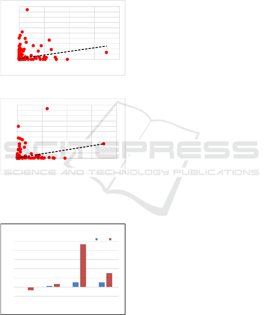
the estimation of radar rain using the Z-R Marshall-

Palmer relation at 4 AWS locations. Based on Figure

4, radar rainfall estimates tend to underestimate

rainfall estimates, this can be seen from the

downward trend line..

Figure 3. Scatter plot of estimated MLP rainfall and AWS

rainfall

Figure 4. Scatter plot of estimated radar rainfall and AWS

rainfall

ME value of a model, used to determine the tendency

of the model in making estimates. The disadvantage

of using ME verfication is that one error can cover the

other's errors due to averaged error.

Figure 5. Comparison of MLP and Radar error values

Some relevant research methods use verification

methods to evaluate the results of models that have

been developed. An important aspect of the error

metric used for model evaluation is its ability to

distinguish between model results. A more

discriminating measure that results in higher variation

in model performance metrics among various sets of

model results is often more desirable. In this case,

MAEs may be influenced by a large number of

average error values without adequately reflecting

some large errors, RMSE is usually better at

expressing model performance differences, but many

researchers choose MAE over RMSE to present their

model evaluation statistics when evaluating the

results of the model (Chai & Draxler, 2014).

In measuring the performance of machine

learning models in this study, the model output will

be validated and verified, that is validating by

measuring the accuracy of the model in predicting the

occurrence and absence of rain and measuring the

accuracy of the model in predicting rain events

according to its category; while in verifying the

model, you will see the model error from the value of

mean error (ME), mean absolute error (MAE), mean

square error (MSE) and root mean square error

(RMSE). MAE is suitable for describing evenly

distributed errors, whereas for normally distributed

errors, RMSE is a better metric to present than MAE.

ME value, is a bias value that can measure the

tendency of the model in the form of underestimate if

it is negative or overestimate is positive, but ME has

a disadvantage because the error values can overlap.

The MSE value can be analogized as a variant plus

the bias squared of a model

Figure 5 shows the comparison of error values

between estimated Radar and MLP rain, the error

value closest to zero is MLP, ie with ME, MAE, MSE

and RMSE values of -0.02 mm / h, 0.25 mm / h, 1.05

mm / h and 1.03 mm / h, while the ME, MAE, MSE

and RMSE values of the radar rain estimate are -0.69

mm / h, 0.69 mm / h, 9.33 mm / h and 3.05 mm / h.

Based on the error value of the ME, MAE, MSE

and RMSE values of the MLP model shown in Figure

5, the MLP model error values compared with the

radar rainfall estimation results, the MLP model error

values are smaller than the radar error values. this

shows that the performance of the MLP model is

better than the results of the estimation of radar

rainforest and the MLP model is able to improve the

rainfall estimation results from the single polarization

radar data in Yogyajarta.

0 5 10 15 20

estimaterainfallfromMLP

rainfallintheground(mm/h)

0 5 10 15 20

estimaterainfallfromradar

rainfallintheground(mm/h)

‐0,02

0,25

1,05

1,03

‐0,69

0,69

9,33

3,05

‐2,00

0,00

2,00

4,00

6,00

8,00

10,00

ME MAE MSE RMSE

ComparisonofMLPandRadarerrors(mm/h)

MLP Radar

Machine Learning System for Rainfall Estimates from Single Polarization Radar

REFERENCES

A. Armoto, L. Fanucci, E.P. Scilingo and D.De Rossi.

(2011). Low-error digital hardware

implementation of artificial neuron activation

functions and their derivative. Microprocessors

and Microsystems, 557-567.

Adi, S. (2013). Characterization of flashflood disaster

in Indonesia. Jurnal Sains dan Teknologi

Indonesia , Vol.15 no 1.

Ali, A and Hidayati,S. (2016). Whirl Wind Detection

and Identification in Indonesia Utilizing Single

Polarization Doppler Weather Radar Volumetric

Data. The International Archives of the

Photogrammetry, Remote Sensing and Spatial

Information Sciences, Volume XLI-B8, 2016

XXIII ISPRS Congress.

Bock, S., & Weis, M. (2019). A Proof of Local

Convergence for the Adam Optimizer.

Proceedings of the International Joint Conference

on Neural Networks, 2019-July(July), 1–8.

https://doi.org/10.1109/IJCNN.2019.8852239

Bringi, V. N. and Chandrasekar, V. (2001). The

polarimetric basis for characterizing precipitation.

In: Polarimetric Doppler Weather Radar.

Cambridge University Press, Cambridge, pp.

378–533.

Chai, T., & Draxler, R. R. (2014). Root mean square

error (RMSE) or mean absolute error (MAE)? -

Arguments against avoiding RMSE in the

literature. Geoscientific Model Development,

7(3), 1247–1250. https://doi.org/10.5194/gmd-7-

1247-2014

Chandrasekar, V., Tan, H., and Chen, H. (2017). A

machine learning system for rainfall estimation

from spaceborne and ground radars. URSI GASS,

mONTREAL.

Codo, M., and Rico-Ramirez, M.A. (2018). Ensemble

Radar-Based Rainfall Forecasts for Urban

Hydrological Applications. Geosciences, Basel

Vol. 8, Iss. 8.

Germann, U., Galli, G. Boscacci, M., and Bolliger,

M. (2006). Radar precipitation measurement in a

mountainous region. Q. J. R. Meteorol. Soc, 132,

1669–1692.

Harrison,D.L., Driscoll,S.J., and Kitchen,M . (2000).

Improving precipitation estimates from weather

radar using quality control and correction

techniques. Meteorol. Appl., 2000, 7, 135–14.

Hornik, K., Stinchcombe, M., & White, H. (1989).

Multilayer feedforward networks are universal

approximators. Neural Networks, 2(5), 359–

366. https://doi.org/10.1016/0893-

6080(89)90020-8

Kingma, D. P., & Ba, J. L. (2015). Adam: A method

for stochastic optimization. 3rd International

Conference on Learning Representations, ICLR

2015 - Conference Track Proceedings, 1–15.

M. Marzuki, H. Hashiguchi, M. K. Yamamoto2, S.

Mori and M. D. Yamanaka. (2013). Regional

variability of raindrop size distribution over

Indonesia. Annales Geophysicae, 31, 1941–1948.

Minervino, A.C and Duarte, E.C. (2015). Loss and

damage affecting the public health sector and

society resulting from flooding and flash floods in

Brazil between 2010 and 2014 - based on data

from national and global information systems.

Ciência & Saúde Coletiva, 685-693.

Paul, S.H., Sharif, H.O., and Crawford, A.M.G.

(2018). Fatalities Caused by Hydrometeorological

Disasters in Texas. MDPI Basel , Vol. 8, Iss. 5.

Raghavan, s. (2003). Radar Meteorology.

Netherlands: Kluwer Academic Publishers.

Rauber, R.M and Nesbitt, S.W. (2014). Radar

Meteorology. LCCN 2017061104 (ebook) .

Rico-Ramirez, M.A., and Cluckie, I.D. (2007).

Bright-band detection from radar vertical

reﬂectivity proﬁles. Int. J. Remote Sens, 28, 4013–

4025.

Tan, H., Chandrasekar, V., & Chen, H. (2017). A

machine learning model for radar rainfall

estimation based on gauge observations. 2017

United States National Committee of URSI

National Radio Science Meeting, USNC-URSI

NRSM 2017, 1–2.

https://doi.org/10.1109/USNC-URSI-

NRSM.2017.7878317

Theodoridis, S., Koutroumbas, K., Koutroumbas, K.,

& Koutroumbas, K. . (2008). Pattern recognition.

Retrieved from http://ebookcentral.proquest.com

Created from indonesiau-ebooks on 2019-03-10

14:16:34.

Tjasyono, B.H.K., and Harijono, S.W.B. (2007).

Meteorologi Indonesia 2. . Jakarta: Badan

Meteorologi dan Geofisika.

Tsun-Hua, Y., Lei, F., and Lung-Yao, C., . (2016).

Improving radar estimates of rainfall using an

input subset of artificial neural networks. J. Appl.

Remote Sens, 10(2), 026013 doi: 10.1117/1.

JRS.10.026013.

Zhang, Z. (2019). Improved Adam Optimizer for

Deep Neural Networks. 2018 IEEE/ACM 26th

International Symposium on Quality of Service,

IWQoS 2018, 1–2.

https://doi.org/10.1109/IWQoS.2018.8624183

CONRIST 2019 - International Conferences on Information System and Technology