Collaboration of Power Suppliers in East Kalimantan using Single

Echelon Economic Dispatch

Wahyuda

, Muslimin

and Samdito Unggul Widodo

Universitas Mulawarman

PT. PLN, Samarinda, Indonesia

Keywords: Transportation Problem, Economic Dispatch, Optimization, Electricity, Collaboration.

Abstract: The Transportation Model, which has been widely applied in the allocation and distribution of goods, has not

been able to be used for the allocation and distribution of electricity. This is because there are differences

between the electrical properties and the properties of the goods. The first difference is that electricity cannot

be saved; this difference causes excess production to be wasted. The second difference is that electricity must

always be available at all times. Power plant scheduling usually uses economic dispatch, but this model has

not considered optimization in transmission and distribution networks. Therefore, this research proposes a

new model called the Single Echelon Economic Dispatch (SEED). This model is a combination of the

transportation model and the economic dispatch model. This model is able to do a joint optimization between

the production and transmission/distribution sides. The SEED model is used to develop a collaboration

strategy between electricity suppliers in East Kalimantan. Simulation results with cost parameters: The best

collaboration when the load is low is PLN + IPP, while at the peak load, the best collaboration is the Joint of

all electricity suppliers.

1 INTRODUCTION

East Kalimantan has four electricity suppliers,

namely PLN, IPP, Leasing, and Excess Capacity.

Each supplier has a different power plant

characteristic. These characteristics cause differences

in fuel costs and emissions (Mahdi et al., 2018;

Muslimin et al., 2019).

The level of fuel consumption is directly

proportional to the level of production, where more

electricity production, the more fuel is used. While

fuel costs and production levels are not directly

proportional but rather form a quadratic equation

(Bhattacharjee and Khan, 2018; Wahyuda et al.,

2018; Gani et al., 2019). The relationship between

variables in the fuel cost function is what causes the

optimization of fuel costs at the power plant to be

optimized.

The level of production is influenced by the

amount of demand and the number of losses in the

transmission network. Losses are directly

proportional to distance, where the longer the

distance, the greater the losses that occur in the

transmission network. Determination of the level of

production is usually done by economic dispatch

2017; Zhou et al., 2017). However, the economic

dispatch model has not considered optimization on

the transmission side. Transmission side optimization

is used to reduce total production costs caused by the

long distance from the plant to the customer.

Therefore, this study proposes Single Echelon

Economic Dispatch, which is a model that is able to

do a combined optimization between the production

and transmission sides. The output of this model can

be used to determine the collaboration strategy

between electricity suppliers in East Kalimantan so

that a lower cost is obtained.

2 LITERATURE REVIEW

2.1. Single Echelon Transportation

Model

The transportation model is first discussed in

(Hitchcock, 1941). In the article, a commodity can be

sent from various sources to various destinations.

This can be seen through the following picture:

Wahyuda, ., Muslimin, . and Widodo, S.

Collaboration of Power Suppliers in East Kalimantan using Single Echelon Economic Dispatch.

DOI: 10.5220/0009403700210028

In Proceedings of the 1st International Conference on Industrial Technology (ICONIT 2019), pages 21-28

ISBN: 978-989-758-434-3

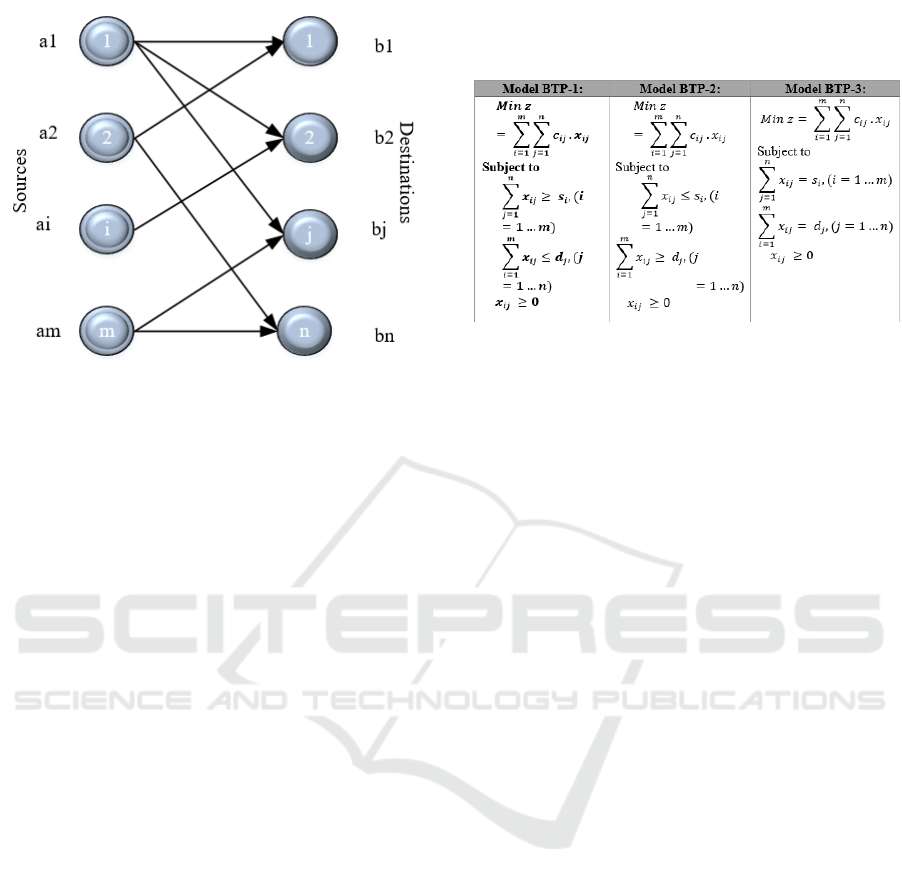
Figure 2.1. The basic concept of the transportation model is

m source n destination.

Figure 2.1 provides an illustration of how the

transportation model works. In general, the

transportation model divides the problem into two

groups, namely the source group and the destination

group. The source can consist of one or several

members, as well as Destination. The transportation

model used to calculate transmission costs can be

seen in (Pablo et al., 2009) illustrated in (Daskin,

1995) as follows:











2.1

Constraints











∀2.2











∀2.3





 0∀,2.4

Where;





= Supply capacity at source i





= Demand at point j.





= Shipping costs from source i to destination j.





= Number of items sent from source i to

destination j.

The main difference between transportation for

goods and transportation for electricity is the balance

between supply and demand. In the transportation

model for goods, suppliers are allowed to send goods

greater than demand, but in transportation for

electricity, suppliers must send goods as big as

demand or called equilibrium. This equilibrium point

is called the Balanced Transportation Problem (BTP)

(Sabbagh et al., 2015). The difference between the

two also occurs in the limits of supplier capacity. The

boundary for transporting goods is simpler than the

economic dispatch limit.

Figure 2.2. Three variations of the Balanced Transportation

Problem (BTP)

Where;





:shippingcostsfromsourceitodestinationj





:thenumberofitemssentfromsourceito

destinationj





:themaximumamountofsupplyofresourcesi





:demandatdestinationj.

2.2. Model of Economic Dispatch

Economic dispatch was introduced since 1928. There

are 3 researchers who are considered as the originator

of the economic principle of the generator (Estrada,

1930; Stahl, 1931; Wilstam, 1928). The initial

economic dispatch is called the classic Economic

dispatch model. This model uses the concept of the

baseload method and the best point load method. How

it works, sort generator units based on the highest

efficiency level. Furthermore, generator scheduling is

given to the generating unit with the highest level of

efficiency, and so on until the last generating unit.

When there are differences in the characteristics

of each plant, the baseload technique becomes less

effective. Therefore, a new technique emerged known

as equal incremental cost. The main concern of this

technique is the characteristics of each different

generator. The way it works, the meeting point of all

generators is searched, and the optimal allocation is

made based on this meeting point. This equal

incremental cost technique is still used today. This

technique was introduced by (Steinberg & Smith,

1933). The advantage of this technique is that it can

provide a low total cost for all the plants involved in

the system. However, this initial model still has

shortcomings, namely the losses in the transmission

network have not been considered. One of the causes

of losses in transmission networks is the length of the

ICONIT 2019 - International Conference on Industrial Technology

transmission network. The longer the transmission

distance, the greater the losses will occur. These

losses will ultimately affect the total cost of fuel

because the plant must produce more electricity than

the demand for compensation losses. Furthermore,

Economic dispatch that considers losses in the

network is introduced by (George et al., 1949). The

Economic Dispatch formula is as follows:



























2.5













2.6









+ Losses 2.7

3 PROPOSED MODEL

Transportation Model has advantages in the field of

distribution. The use of this model causes the total

shipping costs to be minimal. While the Economic

Dispatch model has an advantage in the field of

generator loading allocation or generator scheduling.

The use of economic dispatch models is able to create

a power plant scheduling that results in minimal fuel

costs. Combining the advantages of these two models

provides several advantages. First, the development

of a new transportation model called the Single

Echelon Economic Dispatch (SEED). Second, the

combined optimization between the generator side

and the distribution side. Conceptually, the

development of the SEED model can be seen in the

following figure:

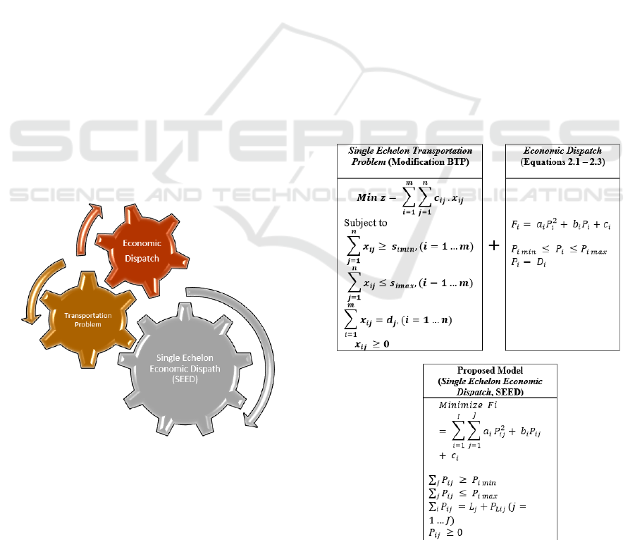
Figure 3.1. Conceptual Model for Single Echelon

Economic Dispatch (SEED) development

Figure 3.1.a conceptually illustrates that the SEED

model is formed from two models, namely the

transportation model and the economic dispatch

model. Figure 3.1.b. is a conceptual model of the

transportation model. While Figure 3.1.c is an

economic dispatch conceptual model. In the same

way, both models are used for resource allocation.

While the difference is in the object faced, where

transportation is commonly used in people or goods

while ED is used in electricity. The nature of the two

objects is different. The main requirement for

electricity is in the form of an equation between the

supply side and the demand side. Therefore, another

approach used is the Balanced Transportation

Problem, as shown in Figure 2.2

Three types of BTP, as shown in Figure 2.2, are

variations of the transportation model application for

real cases. The three variations have the same

objective function, namely minimization of costs

(min z). While the difference between the three is the

model limitation. Cost is the sum of the shipping costs

per unit from each source i to destination j denoted by

multiplied by the number of items sent from source i

to destination j denoted by 



The characteristics of the three variations of BTP

are used as a reference for the development of the

SEED model. Development is carried out by

combining several boundaries so that new variations

of BTP emerge. Furthermore, a merger with the

Economic Dispatch model was obtained to obtain the

SEED model. The result of merging BTP with

economic dispatch as in figure 3.2

Figure 3.2 Schematic of SEED formation

Collaboration of Power Suppliers in East Kalimantan using Single Echelon Economic Dispatch

The SEED model has the objective function of

minimizing fuel costs as well as in the economic

dispatch model. While the difference between them

lies in the coverage of the model. This can be seen

from the notation used. The basic model of economic

dispatch uses notation 



which means the amount of

electricity produced at the generator i. Whereas the

SEED model uses notation 



which means the

amount of electricity produced by the generator i sent

to destination j. If this scope is included in the

objective function, then this model is prepared to be

able to complete two tasks, namely production

optimization tasks, and simultaneous distribution

optimization tasks. As a guarantee of a feasible

solution, the SEED model is also equipped with three

constraints.

4 RESULT AND ANALYSIS

4.1 Experiments

Experiments were carried out on five electricity

supplier cooperation scenarios. Scenario 1 only uses

PLN's power plants. Scenario 2 uses PLN's and IPP's

power plants. Scenario 3 uses PLN's power plants and

Leases. Scenario 4 uses PLN's power plant and

Excess Capacity. Scenario 5 uses PLN's power plants,

IPP, Leases, and Excess Capacity

4.1.1 Scenario 1

In this scenario, there are 11 PLN-owned power

plants that can be used to supply electricity demand.

This scenario has a supply of 346.6 MW. Demand at

low load is 194.9 MW while at peak load is 343.4

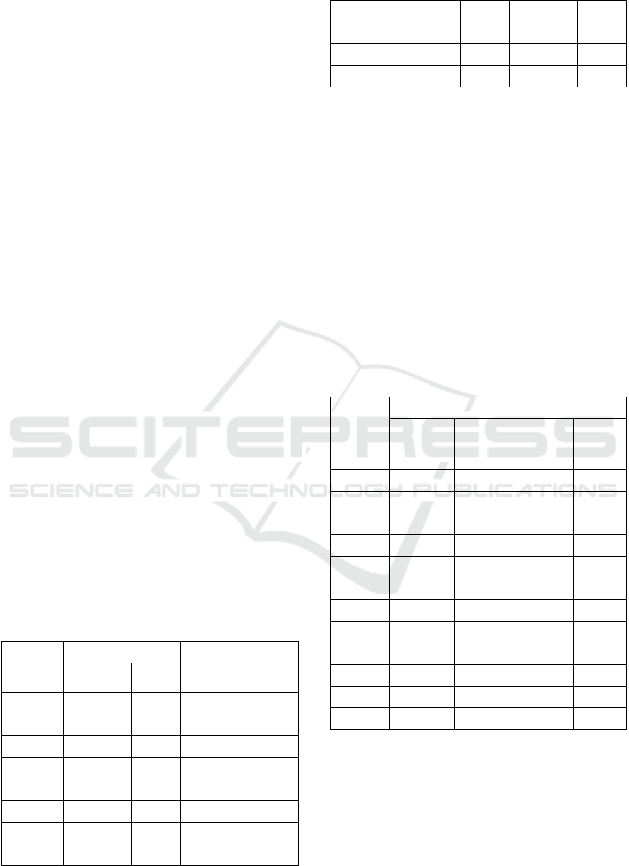
Table 4.1. SEED Model Simulation Results for scenario 1

Power

Plant

Low Peak

Supply

(MW)

Util.

(%)

Supply

(MW)

Util.

(%)

P1 23.5 100.0 23.5 100.0

P2 16.0 100.0 16.0 100.0

P3 3.1 100.0 3.1 100.0

P4 3.6 100.0 3.6 100.0

P5 7.8 100.0 7.8 100.0

P6 14.2 100.0 14.2 100.0

P7 56.8 87.5 65.0 100.0

P8 10.0 100.0 10.0 100.0

P9 2.4 100.0 2.4 100.0

P10 1.0 100.0 1.0 100.0

P11 56.8 28.4 199.2 99.6

Total 195.2 345.8

Based on table 4.1, there is a difference between

supply and demand. At low load, there is a difference

of 0.4 MW while at peak load, there is a difference of

2.4 MW. At low load, there are two power plants

whose production capacity is not used fully, namely

P7 and P11. Whereas during peak loads, only the P11

power plant does not have the entire production

capacity used.

4.1.2 Scenario 2

In scenario 2, there are 11 PLN-owned power plants

and 2 IPP plants that can be used to supply electricity

demand. This scenario has a supply of 523.6 MW.

Demand at low load is 194.9 MW while at peak load

is 343.4 MW.

Table 4.2. SEED Model Simulation Results for scenario 2

Power

Plant

Low Peak

Supply

(MW)

Utiliz.

(%)

Supply

(MW)

Utiliz.

(%)

P1 19.4 82.7 23.5 100.0

P2 16.0 100.0 16.0 100.0

P3 3.1 100.0 3.1 100.0

P4 3.6 100.0 3.6 100.0

P5 7.8 100.0 7.8 100.0

P6 14.2 100.0 14.2 100.0

P7 19.4 29.9 42.7 65.8

P8 8.5 85.1 10.0 100.0

P9 2.4 100.0 2.4 100.0

P10 1.0 100.0 1.0 100.0

P11 20.0 10.0 42.7 21.4

P24 20.7 25.2 82.0 100.0

P25 58.9 62.0 95.0 100.0

Based on table 4.2, there is a difference

between supply and demand. At low load, there is a

difference of 0.2 MW while at high load, there is a

difference of 0.6 MW. At low loads, there are six

power plants whose production capacity is not used at

all. Whereas during peak loads, there are two power

plants whose production capacity is not fully utilized.

ICONIT 2019 - International Conference on Industrial Technology

4.1.3 Scenario 3

In scenario 3, there are 11 PLN-owned power plants

and five rental plants that can be used to supply

electricity demand. This scenario has a supply of

419.1 MW. Demand at low load is 194.9 MW while

at peak load is 343.4 MW

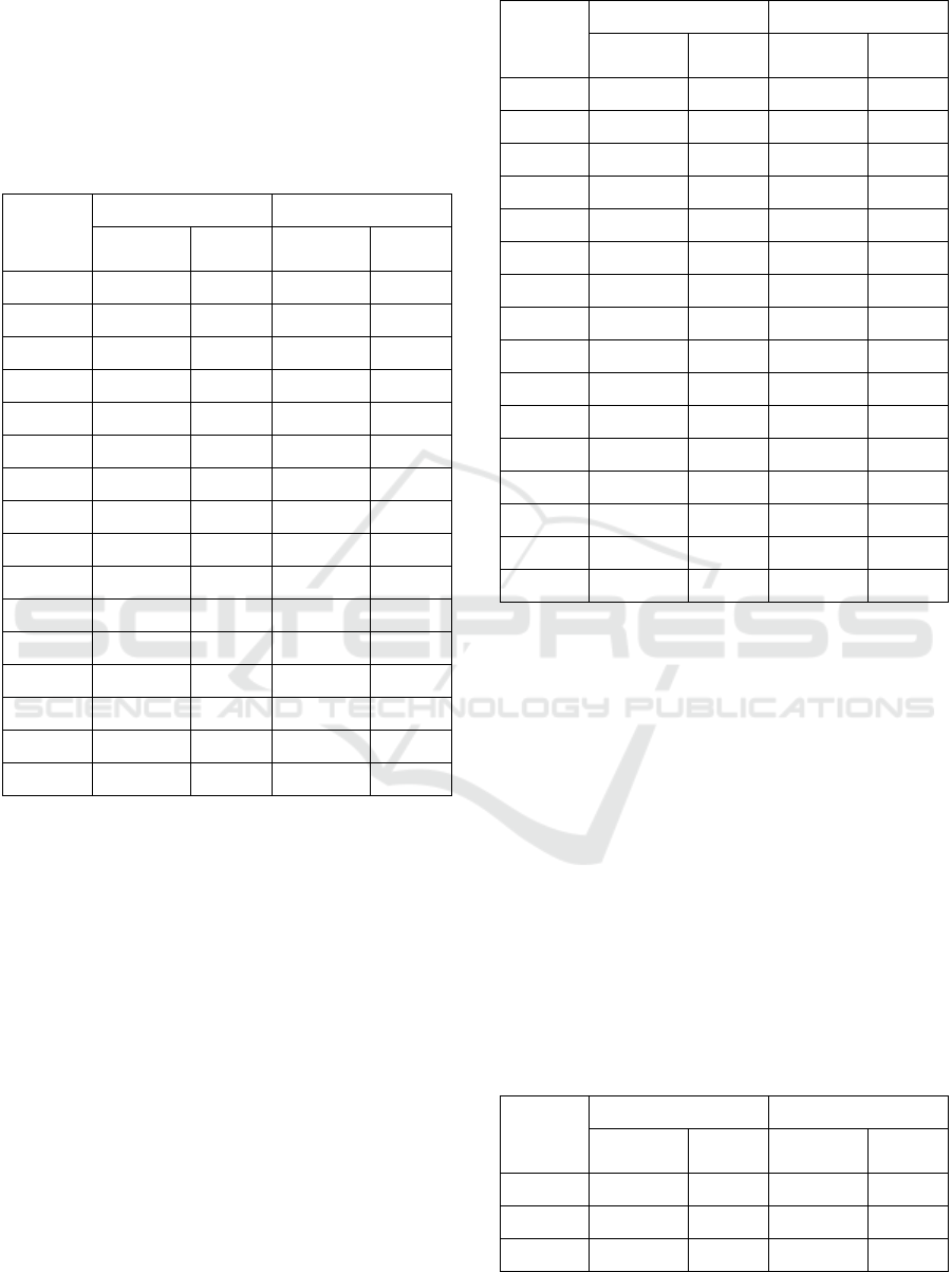
Table 4.3. SEED Model Simulation Results for scenario 3

Power

Plant

Low Peak

Supply

(MW)

Utiliz.

(%)

Supply

(MW)

Utiliz.

(%)

P1 23.5 100.0 23.5 100.0

P2 16.0 100.0 16.0 100.0

P3 3.1 100.0 3.1 100.0

P4 3.6 100.0 3.6 100.0

P5 7.8 100.0 7.8 100.0

P6 14.2 100.0 14.2 100.0

P7 28.9 44.5 65.0 100.0

P8 10.0 100.0 10.0 100.0

P9 2.4 100.0 2.4 100.0

P10 1.0 100.0 1.0 100.0

P11 28.9 14.5 125.1 62.5

P12 12.0 55.8 21.5 100.0

P13 32.5 81.3 40.0 100.0

P14 2.7 100.0 2.7 100.0

P15 5.7 100.0 5.7 100.0

P16 2.6 100.0 2.6 100.0

Based on table 4.3, there is a difference between

the amount of supply and demand. At low load, there

is a difference of 0.1 MW while at peak load, there is

a difference of 0.8 MW. At low loads, there are four

power plants whose production capacity is not used at

all. Whereas during peak loads there is only one

power plant whose production capacity is not fully

utilized

4.1.4 Scenario 4

In scenario 4, there are 11 PLN-owned power plants

and 5 Excess Capacity plants that can be used to

supply electricity demand. This scenario has a supply

of 391.4 MW. Demand at low load is 194.9 MW

while at peak load is 343.4 MW

Table 4.4. SEED Model Simulation Results for scenario 4

Power

Plant

Low Peak

Supply

(MW)

Utiliz.

(%)

Supply

(MW)

Utiliz.

(%)

P1 23.5 100.0 23.5 100.0

P2 16.0 100.0 16.0 100.0

P3 3.1 100.0 3.1 100.0

P4 3.6 100.0 3.6 100.0

P5 7.8 100.0 7.8 100.0

P6 14.2 100.0 14.2 100.0

P7 34.3 52.8 65.0 100.0

P8 10.0 100.0 10.0 100.0

P9 2.4 100.0 2.4 100.0

P10 1.0 100.0 1.0 100.0

P11 34.3 17.1 136.2 68.1

P17 6.8 100.0 6.8 100.0

P19 5.0 100.0 5.0 100.0

P20 22.0 100.0 22.0 100.0

P22 6.0 100.0 6.0 100.0

P23 5.0 100.0 5.0 100.0

Based on table 4.4, there is a difference between

the amount of supply and demand. At low load, there

is a difference of 0.13 MW while at peak load, there

is a difference of 1.04 MW. At low loads, there are

two power plants whose production capacity is not all

used. Whereas during peak loads, there is only one

power plant whose production capacity is not fully

utilized.

4.1.5 Scenario 5

In scenario 5, there are 11 PLN power plants, 2 IPP

plants, five rental plants, and 5 Excess Capacity

plants, which can be used to supply electricity

demand. This scenario has a supply of 391.4 MW.

Demand at low load is 194.9 MW while at peak load

is 343.4 MW

Table 4.5. SEED Model Simulation Results for scenario 5

Power

Plant

Low Peak

Supply

(MW)

Utiliz.

(%)

Supply

(MW)

Utiliz.

(%)

P1 14.0 59.6 19.5 82.9

P2 16.0 100.0 16.0 100.0

P3 3.1 100.0 3.1 100.0

Collaboration of Power Suppliers in East Kalimantan using Single Echelon Economic Dispatch

P4 2.0 55.6 3.6 100.0

P5 7.8 100.0 7.8 100.0

P6 8.3 58.2 14.2 100.0

P7 8.3 12.7 19.5 30.0

P8 7.0 70.0 8.5 85.5

P9 2.4 100.0 2.4 100.0

P10 1.0 100.0 1.0 100.0

P11 20.0 10.0 20.0 10.0

P12 12.0 55.8 12.0 55.8

P13 32.5 81.3 32.5 81.3

P14 2.7 100.0 2.7 100.0

P15 2.3 40.9 5.7 100.0

P16 2.6 100.0 2.6 100.0

P17 1.0 14.7 6.8 100.0

P19 0.0 0.0 5.0 100.0

P20 10.0 45.5 22.0 100.0

P22 1.0 16.7 6.0 100.0

P23 1.0 20.0 5.0 100.0

P24 20.0 24.4 32.8 40.0

P25 20.0 21.1 95.0 100.0

Based on table 4.5, there is a difference between

the amount of supply and demand. At low load, there

is a difference of 0.1 MW while at peak load, there is

a difference of 0.26 MW. At low loads, there are 60%

power plants whose production capacity is not used at

all. Whereas during peak loads there are only 30%

power plants whose production capacity is not fully

utilized

4.2 Analysis

The SEED model succeeded in scheduling a more

detailed power plant and distribution. Power plant

scheduling is done using the economic dispatch

model. In addition to scheduling a power plant, the

SEED model also simultaneously optimizes

distribution lines and losses as well as the goal of

minimizing total fuel costs. The total fuel cost is

influenced by the characteristics of the plant, the

amount of electricity demand, and losses in the

transmission/distribution network. The longer the

distance that must be traveled by electricity from the

generator to the customer, the greater the losses that

will occur. In this case, the losses on the

transmission/distribution network are affected by

mileage.

Minimizing losses can be an effort to reduce total

fuel costs. However, minimizing losses does not

always produce the smallest total cost. This can occur

due to different generator characteristics. If the

electric power system has the same generator

characteristics, reducing losses will automatically

reduce the total fuel cost.

Based on experiments using five scenarios, it is

known that: Scenario 1: If losses can be minimized,

PLN's power plants are able to meet electricity

demand at low load and peak load. Electricity demand

during peak load is 343.4 MW, while the production

capacity of all PLN-owned power plants is 346.6

MW, meaning that if losses on the entire transmission

network can be reduced below 3.2 MW, the PLN-

owned power plant can serve demand at the time peak

load. However, if losses cannot be controlled, then the

electricity demand must be supplied from other plants

through a cooperation mechanism. Cooperation

between generators as electricity suppliers must be

calculated in detail. This is due to differences in the

characteristics and location of each power plant

owned by electricity suppliers. Differences in

generator characteristics cause differences in total

fuel costs and emissions.

Based on the simulation results for scenario 2,

cooperation between PLN's power plant and IPP can

supply electricity during low load and peak load. This

is because the combined production capacity of PLN

+ IPP is greater than the total demand and losses.

When the load is low, the production capacity of PLN

and IPP's power plants is used in a balanced manner.

During peak load, all IPP's power plant production

capacity is used, while PLN's power plant production

capacity is 55% used. Although the percentage of

PLN's power plant capacity usage is smaller, losses

and emissions generated are greater than IPP's.

In scenario 3, cooperation between PLN's power

plants and rental plants can meet electricity during

low and peak loads. As a percentage, the cooperation

between the two prioritizes the use of rental power

plants compared to PLN's power plants during peak

loads, the production capacity of rental plants is used

entirely

In scenarios 4 and 5, the same pattern is found.

Production priority is always given to the Excess

capacity generator. Even in scenario 4, both under

low load and peak load conditions, the Excess

Capacity generator is the main generator.

In general, it can be said that PLN's power plants

are the ones with the lowest fuel costs. This can be

seen in the utilization of plants, which are almost

always 100%. However, the production capacity of

PLN's power plants has never been used at 100%. In

ICONIT 2019 - International Conference on Industrial Technology

the case of optimization with the objective function

of minimizing fuel costs, the use of production

capacity reaching 100% means that the power plant

becomes the main priority because it has the lowest

total fuel cost compared to other plants. Such

conditions are an impact of the characteristics of

power plants. This characteristic difference causes

P11 to be the only PLN-owned power plant, which is

the last choice in the allocation of loading because

this plant requires more expensive fuel costs. The use

of P11 generators is possible when serving peak

loads.

Based on the five scenarios above, determining

the best scenario depends very much on the

considerations used by the decision-maker. This is

because the selection of the best scenario based on the

lowest cost will increase emissions, and vice versa.

Not only that, but the best scenario based on cost

minimization also depends on the condition of the

electricity load during low load or peak load.

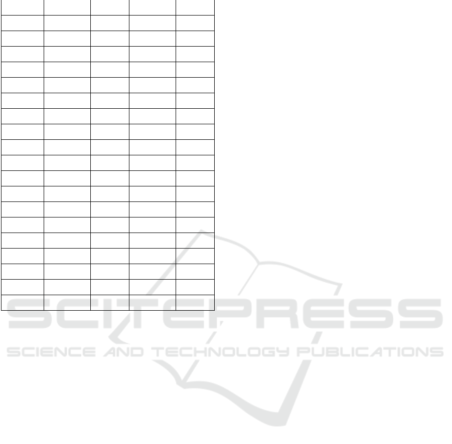
When the load is low, the best scenario is scenario

2. This scenario is the allocation of PLN and IPP's

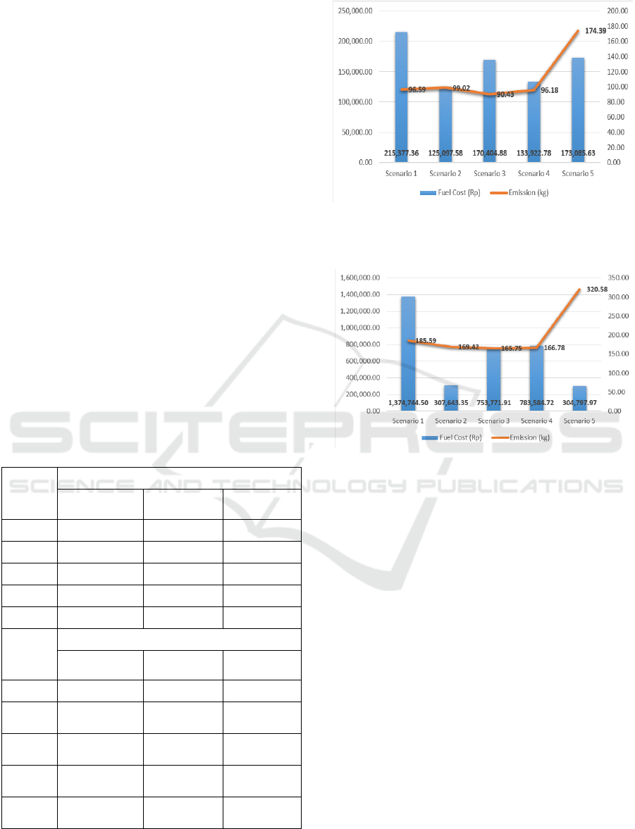
power plant loading. Whereas during peak load, the

best scenario is scenario 5. Scenario 5 is the allocation

of loading with a combined power plant as the best

parameter is the smallest cost.

Table 4.6. Comparison Between Scenarios for Peak load

and low load conditions

Scenari

Low

Fuel Cost

(Rp)

Emission

(kg)

Losses

(MW)

1 215,377.36 96.59 0.36

2 125,097.58 99.02 0.21

3 170,404.88 90.43 0.10

4 133,922.78 96.18 0.13

5 173,085.63 174.39 0.10

Scenari

Peak

Fuel Cost

(Rp)

Emission

(kg)

Losses

(MW)

1 1,374,744.50 185.59 2.36

307,643.

35 169.42 0.64

753,771.

91 165.75 0.80

783,584.

72 166.78 1.04

304,797.

97 320.58 0.26

Figure 4.1: Comparison between scenarios with parameters

Fuel costs and emissions under low load conditions

Figure 4.2: Comparison between scenarios with parameters

Fuel costs and emissions under Peak Load conditions

5 CONCLUSIONS

The SEED model is a new variation of the

transportation model. SEED is a combination of the

transportation model with the economic dispatch

model. The combination of these two models causes

the transportation model can be used for the

allocation of electricity production and distribution.

SEED is able to optimize the combination of

production and distribution. The output of the SEED

model is the allocation of power plants, the

distribution of electricity from a source to a

destination, the distance of electricity from the plant

to the customer, losses incurred by each plant and

emissions

In the case of the centralization of electricity using

the SEED model, the allocation of loading is divided

into two conditions, namely low load and peak load.

When the load is low, the best allocation of expenses

from a cost perspective is a collaboration between

PLN's power plant and IPP. However, this choice will

have an impact on increasing emissions and losses.

Collaboration of Power Suppliers in East Kalimantan using Single Echelon Economic Dispatch

The combination of these two plants generates greater

emissions and losses when compared to the other

three scenarios, namely scenario 1 (only using PLN's

power plant), scenario 3 (combined PLN and Lease),

and scenario 4 (combined PLN and EC). Whereas

during peak load, the best allocation of expenses from

the standpoint of costs and losses is when using

scenario 5, which is a combination of all power plants

belonging to all parties in the Mahakam system.

However, the selection of this scenario has the worst

impact on the environment because the emissions

produced are highest when compared to the other four

scenarios

ACKNOWLEDGMENTS

This research was funded by the Directorate of

Higher Education Ministry of National Education

Republic of Indonesia Fiscal Year 2019.

REFERENCES

Bhattacharjee, V. and Khan, I. (2018) ‘A non-linear convex

cost model for economic dispatch in microgrids’,

Applied Energy. Elsevier, 222(January), pp. 637–648.

doi: 10.1016/j.apenergy.2018.04.001.

Gani, I. et al. (2019) ‘Analysis of costs and emissions on

the addition of production capacity of the power plant

using multi echelon economic dispatch Analysis of

Costs and Emissions on The Addition of Production

Capacity of The Power Plant Using Multi Echelon

Economic Dispatch’, in AIP Conference Proceedings.

doi: 10.1063/1.5112487.

Mahdi, F. P. et al. (2018) ‘A holistic review on optimization

strategies for combined economic emission dispatch

problem’, Renewable and Sustainable Energy Reviews.

Elsevier Ltd, 81(March 2017), pp. 3006–3020. doi:

10.1016/j.rser.2017.06.111.

Muslimin, Wahyuda and Tambunan, W. (2019)

‘Cooperation between power plant in East Kalimantan

by integrating renewable energy power plant

Cooperation between power plant in East Kalimantan

by integrating renewable energy power plant’, in IOP

Conference Series: Materials Science and Engineering.

doi: 10.1088/1757-899X/528/1/012080.

Wahyuda, Santosa, B. and Rusdiansyah, A. (2017) ‘Load

allocation of power plant using multi echelon economic

dispatch’, in AIP Conference Proceedings. doi:

10.1063/1.5010624.

Wahyuda, Santosa, B. and Rusdiansyah, A. (2018) ‘Cost

analysis of an electricity supply chain using

modification of price based dynamic economic dispatch

in wheeling transaction scheme’, in IOP Conference

Series: Materials Science and Engineering. doi:

10.1088/1757-899X/337/1/012009.

Zhou, J. et al. (2017) ‘A multi-objective multi-population

ant colony optimization for economic emission

dispatch considering power system security’, Applied

Mathematical Modelling, 45, pp. 684–704. doi:

10.1016/j.apm.2017.01.001.

ICONIT 2019 - International Conference on Industrial Technology