
Artificial Neural Network and Its Application in Medical Disease
Prediction: Review Article
Putri Alief Siswanto
1
and Riries Rulaningtyas
2
1
Biomedical Engineering Graduate Program, Faculty of Science and Technology, Airlangga University,
Surabaya, Indonesia
2
Department of Physics, Faculty of Science and Technology, Airlangga University, Surabaya, Indonesia
Keywords: Artificial Neural Network, Prediction, Regression.
Abstract: Artificial Neural Network (ANN) has gained considerable attention in many fields, including medicine.
Despite this, many physicians are still oblivious to the concept of ANN. In this paper, therefore, we attempt
to provide an overview of the features of ANN. In addition, performance comparison in medical disease
prediction between ANN and regression as a standard statistical technique is also conducted. This is due to
the proficiency of ANN in modeling complex, non-linear relationships which makes it highly attractive for
diagnostic or prognostic purposes. It can be concluded that ANN has similar performance to, and in some
cases, is better than regression.
1 BACKGROUND
In the last few decades, artificial intelligence (AI) has
gained increasing popularity among researchers. AI is
a new technology in computer science and is
distinguished from conventional computers. Whereas
its counterpart could only perform specific tasks
based on instructions given or often referred as
program (software), AI tries to adopt the flexibility of
the human brain (Sazli, 2006).
One of the most popular branches of AI is that of
artificial neural networks (ANN). ANN is an
information processing system that resembles
biological neural networks (Haykin, 2009); ANN has
been used extensively in many disciplines, including
medicine (Ramesh et al., 2004). Despite its potential,
ANN is nevertheless still unknown to many
practitioners. Therefore, we will provide an overview
of ANN that includes definition, components,
architecture, training methods and the
backpropagation method. In the future, it is expected
that not only will more physicians become familiar
with this method, but that they will also be able to
properly apply this method.
The application of ANN is mostly used for
prediction and modeling. In order to provide a more
comprehensive understanding of ANN’s application
in medical disease prediction specifically,
comparative studies of ANN and standard statistical
analysis are also discussed.
2 METHOD
The literature search was conducted using the terms
‘neural network’, ‘prediction’ and ‘regression’ from
the year 2000 to the present. Comparison studies were
limited to medical applications. Titles and abstracts
were reviewed to identify papers that could contribute
to this discussion, and full-text versions were
acquired.
3 DISCUSSION
3.1 Definition of ANN
ANN is a mathematical representation of the human
neural architecture, and reflect its learning and
generalization abilities (Dave and Dutta, 2014). In
ANN, information processing occurs in elements
called neurons. Signals are transmitted from one
neuron to another through connection. Each
connection has a synaptic weight that is multiplied
with the input signal. Each neuron then applies an
Siswanto, P. and Rulaningtyas, R.
Artificial Neural Network and Its Application in Medical Disease Prediction: Review Article.
DOI: 10.5220/0009387400170025
In Proceedings of the 4th Annual International Conference and Exhibition on Indonesian Medical Education and Research Institute (The 4th ICE on IMERI 2019), pages 17-25
ISBN: 978-989-758-433-6
Copyright
c
2020 by SCITEPRESS – Science and Technology Publications, Lda. All rights reserved
17

activation function to the input signal to determine
output (Nicoletti, 2000).
ANN emulates the way the human brain learns
through examples. The brain makes some
adjustments to synaptic connections during the
learning process. This is applied to ANN. During the
learning phase, weights are adjusted to values such
that each input produces desired output (Huang,
2017).
3.2 ANN Architecture
Neurons are organized in layers. Each neuron in a
layer is connected with every other neuron in the
previous or next layer through a synaptic weight. The
values of this weight indicates the strength of the
connection (Richards, 2006).
The structure of the neural network is formed by
an input layer, one or more hidden layers and the
output layer. Network architecture plays a major role
in the success of ANN. Therefore, an optimal network
must be determined (Amato et al., 2012).
The input layer acts as an intermediary between
the network and the outside. Neurons in this layer
only forward data to the following layer, as there are
no data changes being made (Wang et al., 2009).
Information received by neurons in the input layer
are then transfered to the output layer through the
hidden layer; the hidden layer helps network to
recognize still more patterns. The number of hidden
layers depends on the complexity of the system
studied (Sazli, 2006). For most of the biomedical
applications, there is no evidence that suggests that
more than one hidden layer will meaningfully add to
the predictive capabilities of a network (Ahmed,
2005).
The selection of a number of hidden neurons
remains one of the major problems in ANN, since it
is dependent on factors unique to each case. Too
many hidden neurons will cause the network to
overfit, or lose its generalizing ability, since the
network tends to remember all the given examples.
Conversely, if the number of hidden neurons is
smaller than the complexity of the problem, it will
cause the network to underfit and hinder convergence
(Ramli and Clean, 2011)
Convergence is a condition that happens when the
network shows minimal errors after the training
process.The network will stop learning when it
reaches convergence (Sun et al., 2003). Convergency
of target and model output values can be observed
with the use of mean error (BIAS), mean absolute
error (MAE), mean absolute percentage error
(MAPE) and root mean square error (RMSE) (Bilgili
and Sahin, 2010).
Panchal and Panchal (2014) conducted a literature
review regarding the method of selecting a number of
hidden neurons. The hidden layer has significant
influence on the output, although it does not interact
outside of the network. Several approaches are
available to determine the number of hidden neurons,
such as trial and error, rule of thumb and the simple
method. It should be noted that researchers who
proposed some of the methods did not use the results
of the formula in the study they conducted. Therefore,
it is recommended to use trial-and-error methods as
long as there is no accurate guideline regarding the
selection of the number of hidden neurons.
If the network has several hidden layers, the
lowest layer functions to receive input. The value of
the input (Nett) of the j-th neuron in the hidden layer
equals to the number of multiplications between the
weight value (𝑊) and the output value (𝑂) of the i-th
neuron in the previous layer (input neuron) plus bias
(W, jth neuron).
𝑁𝑒𝑡𝑡
𝑊
𝑖𝑗
.𝑂
𝑖
𝑊𝑜𝑗
(1)
Bias is the value of weight which connects bias
neurons and neurons in the next layer. The input of
bias neuron always has a value of 1. Bias neurons can
be added to input layer and hidden layer. Bias can be
initialized randomly within a range of -1 to 1. Bias is
aimed to improve the network’s output to
approximate the desired value (Abiodun et al., 2018).
The output value of neurons in the hidden layer is
a function of the input value f (net(j)). Several choices
for activation functions are available. The same
formulas used in the hidden layer are applied to the
output layer, including the activation function, but
output are considered to be the result of the learning
process (Liang et al., 2010).
There are three types of ANN architecture: single-
layer, multi-layer and competitive-layer. A single-
layer network has a set of neuron inputs directly
connected to a set of outputs, and no hidden layers are
found (Alsmadi et al., 2009). This results in limited
ability while generalizing more complex problems.
To overcome this, a single-layer network adds one or
more hidden layers, or a so-called multi-layer. A
competitive-layer network is similar to a single- or
multi-layer network, but there is feedback from
output neurons towards input throughout the network
(feedback loop) (Nicoletti, 2000).
The 4th ICE on IMERI 2019 - The annual International Conference and Exhibition on Indonesian Medical Education and Research Institute
18
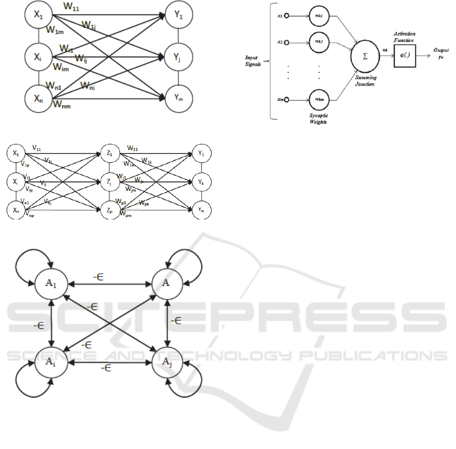
Figure 1: Example of single-layer ANN.
Figure 2: Example of multi-layer ANN.
Figure 3: Example of competitive-layer ANN.
3.3 ANN Components
The basic building block of neural networks is the
neuron. The neuron can be perceived as a processing
unit. In a neural network, neurons are connected with
each other through synaptic weights. Weight stores
information at certain values. Positive values will
strengthen the signal and vice versa.
Each neuron receives weighted information via
these synaptic connections and then passes the
weighted sum of those input signals in order to be
compared with a threshold value using activation
function. If the amount of input exceeds a certain
threshold value, the neuron will be activated and send
its output. If the amount of input is smaller than the
threshold value, the information will not be passed on
(Nicoletti, 2000).
Figure 4: Structure of ANN.
For example, if 𝑥
,𝑥
,…𝑥
is an input neuron and
𝑤
,𝑤
,…𝑤
is synaptic weight to the output
neuron, then the weighted sum will give an output of:
𝑢
𝑥
𝑤
𝑥
𝑤
⋯𝑥
𝑤
(2)
Weights can be randomly initialized in a range value
of -1 to 1 and should be a small value.
The activation function is a function that maps
input to its output. It is not only used to determine the
output of a neuron, but also to modify the output into
a certain range of values so that it can approach
maximum and minimum values, as well (Siang,
2005).
There are several types of activation functions:
the step biner, bipolar, linear and sigmoid functions.
Must-have characteristics for activation functions are
continuous, differentiable, not asymptotic, not
monotonically decreasing and easily calculated
(Richards, 2006).
The step biner function converts input value into
binary output (0 or 1). The bipolar function has an
output result of 1, 0 or -1. A linear function has the
same output value as input value. The sigmoid
function is often used in a backpropagation algorithm
due to its shape of function and easily computed
derivatives. Parameter related to the shape (slope) of
the sigmoid function is alpha (α). The greater the
value, the more the non-linear sigmoid function will
produce.
There are two steps of the ANN: the training and
testing phase. Each step uses different data sets. The
training phase produces the final weight which is later
used in the testing phase (Toshniwal and Alsma,
2009).
There is no exact rule regarding the composition
of training and testing data. Crowther and Cox (2005)
divided training and testing data with a distribution of
70:30 of the total data. Meanwhile, some researchers
divide data with a composition of 80:20 for training
Artificial Neural Network and Its Application in Medical Disease Prediction: Review Article
19

and testing data. Randomization is advised before
dividing the data in order to reduce bias.
There are two important aspects of the training
data set. First, network performance not only depends
on network parameters, but also on the accuracy of
the training data set. Training data should be able to
represent all the inputs which are intended to be
trained in order to precisely produce output (Azmi
and Cob, 2010). Extreme values in data can be well
represented if included in training data, but the
network cannot accurately extrapolate values if it is
outside the training data (Ramli and Clean, 2011).
Second, the data needs to be normalized before being
processed. This aims to simplify the network during
the training phase. Network output is then
denormalized to return to its original value (Jiang et
al., 2010).
In addition to training and testing data, there is
validation data. The validation step is used to
optimize model parameters and monitor network
performance (Lisboa, 2002). Performance of training
and validation data sets will improve during the
training process. But if network capacity is greater,
then performance of validation data set will decrease.
This can be a sign of overlearning or overfitting, and
the training process should be immediately stopped
(early stopping) (Ahangar, 2010).
In general, training data is divided into training
and validation data sets. This validation technique is
called the split-sample method (Park and Han, 2018).
Another popular validation method is n-fold cross-
validation. This method is performed by dividing
training data sets into n data sets. The network is
validated every time the learning process is
completed using different subsets. The training
process is carried out with remaining data sets which
were not being used for validation. Model
performance is measured by calculating the average
RMSE of all validations performed (Almeida, 2002).
Other validation techniques are temporal and
external validation (Park and Han, 2018). Temporal
validation is carried out using the cohort at different
times (Lisboa and Taktak, 2006). External validation
involves a larger database (apart from previously
tested population) (Terrin et al., 2003), which is
usually conducted through multicenter studies.
Testing on a separate data set would have provided an
unbiased estimate of the generalization error
(Ahangar, 2010).
Measures of a network’s performance for
diagnostic or predictive models include discrimina-
tion and calibration. Discrimination determines how
well groups within data are separated. Discrimination
performance is typically measured in terms of
sensitivity, specificity and receiver operating
characteristic (ROC) curve analysis. Calibration
refers to correspondence between predicted and
actual probabilities. It is measured by calculating
accuracy or difference between target and output
value (Park and Han, 2018)
3.4 ANN Training Methods
There are three major categories of the training
method. The first is supervised learning, in which a
network is provided with expected output and trained
to respond correctly through error correction and
weight adjustment. This method is commonly used
for pattern/memory association and regression
analysis/function estimation. Some examples of
applications are pattern recognition (face/object
identification), sequence identification (gestures,
language, handwriting) and decision-making (Ashok
et al., 2010). ANN methods belonging to supervised
learning are Hebb’s rule, Perceptron, the Delta rule,
backpropagation, radial basis function (RBF), and
bidirectional associative memory (BAM) (Ramli and
Clean, 2011).
Second is unsupervised learning, in which the
network is provided with no knowledge of expected
output beforehand and trained to discover structures
in presented inputs. Weights are categorized into a
certain range of values in which nearly same input
will produce same output. It is commonly used for
grouping or classification. ANN methods belonging
to unsupervised learning are self-organizing maps
(SOM) and k-means clustering (KNN) (Kusumadewi,
2006).
The third is reinforcement learning, in which a
network is not provided with explicit output; instead,
it is periodically given performance indicators which
act as a supervisory system (Nayak et al., 2001).
3.5 ANN Backpropagation
The most common type of ANN used is the
backpropagation learning algorithm. The basic theory
of backpropagation is based on the error-correction
learning rule, which uses the error function in order
to modify the connection weights to gradually reduce
the error. Error is the difference between actual output
and the desired output. Therefore, backpropagation is
a supervised learning paradigm because it requires a
desired output (Alsmadi et al., 2009).
There are several methods of weight updates,
including gradient descent, quasi newton (LM) and
genetic algorithm. Gradient descent is used in
The 4th ICE on IMERI 2019 - The annual International Conference and Exhibition on Indonesian Medical Education and Research Institute
20

backpropagation and has better performance
compared to other methods (Ghaffari et al., 2006).
Gradient descent technique is the most common
approach that is utilized in backpropagation. It is
conducted by modifying the weight via values
proportional to the derivative of the error function
(Abiodun et al., 2018).
The disadvantage of the gradient descent method
is that it is likely to get caught up in local minima.
Local minima are when a network achieves an error
that is lower than the surrounding possibilities, but it
is not the smallest possible one. Training that takes
much time but does not give better results is a sign of
local minima.
Backpropagation can be implemented in two
modes, the batch and incremental modes (Aria,
2003). In batch mode, the network weights are
updated once after the presentation of the complete
training set. While in incremental mode, weights are
updated after each pattern presentation. The last mode
is the most frequently used (Sazli, 2006). According
to Ghaffari et al. (2006), there is no significant
difference between the two modes in accuracy, but
batch mode has 3-to-4-times higher convergence
speed than incremental mode.
Backpropagation algorithm can be decomposed in
the following three steps: (a) computation of a feed-
forward stage, (b) backward propagation of the error
to both the output layer and the hidden layers, and (c)
weights update. The algorithm is stopped when the
value of the error function has become less than a
predefined acceptable tolerance (Laudon et al., 2007).
During the feedforward step, each input neuron
(X
i
) will receive a signal input and forward to each
neuron in hidden layer (Z
j
). Each neuron in the hidden
layer then calculates its activation and sends a signal
(z
j
) to each output neuron. Then, each output neuron
(Y
k
) also calculates its activation (y
k
) to produce a
response to the input given by the network.
Each neuron output then compares its activation
(y
k
) with a target value (t
k
) to calculate the error.
Based on that error, 𝛿
is calculated. Factor 𝛿
is used
to distribute errors back to the previous layer.
Meanwhile, factor 𝛿
is used to update weight, which
connects hidden and input layer.
The learning rate is a factor that controls the speed
of the training phase. It is determined through trial
and error to generate the fastest iteration in achieving
convergence (Amin et al., 2012). The input of
learning rate is within range of 0 to 1 (Wilson, 2001).
A too-high value can cause the algorithm to become
unstable due to oscillation of weight update and result
in less generalizing ability. Meanwhile, a too-small
value will result in a longer time to achieve
convergence and lead to local minima (Suliman and
Zhang, 2015).
A maximum epoch is the maximum number of
epochs allowed during the training process. Iteration
will be stopped if epoch in the process exceeds
maximum defined training epochs.
Iteration can also be stopped if network error is
equal to or smaller than the target error. The target
error is a predetermined maximum error value of
network performance. In addition, the training phase
can be stopped if there is no significant weight update
after a long-term process (Ahangar, 2010).
3.6 Application of ANN in Medical
Disease Prediction
In the last decade, the use of AI has become widely
accepted in medical application. This is manifested
by an increasing number of medical devices currently
available on the market that are equipped with AI
features, and also the number of publications in
medical journals (Gant et al., 2001).
ANN is the most well-known method in AI
(Meengoen et al., 2017). Considerable attention has
been paid to the development of ANN and its
application in many areas, including medicine. It is
currently an issue of great interest, especially with
regard to diagnostic or predictive analysis (Amato et
al., 2012). ANN models have been shown to be
valuable tools in reducing the workload on clinicians
by providing decision support (Gant et al., 2001).
Meanwhile, other branches of AI, such as fuzzy
expert systems, evolutionary computation and hybrid
intelligent systems, can be applied to certain clinical
conditions to a limited extent (Ramesh et al., 2004).
ANN models possess such characteristics as:
(a) nonlinearity, which can approximate any non-
linear mathematical function (this is particularly
useful when the relationship between the variables is
too complex and therefore difficult to handle
statistically); (b) noise-insensitivity enables them to
accept a certain amount of uncertain data or
measurement errors without a serious effect on
accuracy; (c) learning and adaptability allows a
network to modify its internal structure (Paliwal and
Kumar, 2009); (d) high parallelism implies fast
processing; and (e) generalization enables application
of the model to untrained data (Ahmed, 2005).
Advantages of using ANN include: (a) less formal
statistical training to develop, (b) having a wide
variety of training algorithms and (c) the ability to
detect complex nonlinear relationships between
variables (Sargent, 2001).
Artificial Neural Network and Its Application in Medical Disease Prediction: Review Article
21

Meanwhile, disadvantages of ANN include:
(a) as they are considered to be ‘black box’ methods,
one cannot exactly understand which interactions are
being modeled in their hidden layers (Mantzaris et al.,
2008); (b) weights produced during the training phase
are lacking in interpretability, and therefore
inferences regarding the significance of certain
variables cannot be drawn (Paliwal and Kumar,
2009); (c) model development is empirical (through
trial and error) and requires lengthy development and
time to optimize, so many methodological issues
therefore remain to be solved (Prieto et al., 2016); (d)
models are susceptible to overfitting; and (e) they are
difficult to apply in certain fields because of
computational requirements (Terrin et al., 2003).
Although there is currently ready-to-use software, it
has not yet been standardized (Sargent, 2001).
There are still only a few published clinical trials
for ANN (Lisboa and Taktak, 2006). Further clinical
trials which are properly designed are needed before
this method finds application in a real clinical setting
(Ramesh et al., 2004).
Neural networks can be applied for complex
pattern recognition, classification problems and
function estimation, but are mostly used for
modelling and prediction. The non-linear structure of
ANN enables us to model complex functional forms
(Paliwal and Kumar, 2009). This suggests that ANN
is a promising method for overcoming non-linear
problems demonstrated in biological systems
(Almeida, 2002).
Prediction models in medicine are used for
diagnostic and prognostic purposes. Research has
been conducted on ANN in medicine intended to
improve the accuracy of clinical predictions (Escobar
et al., 2016). The most common method used for
medical disease prediction is the regression model
(Sargent, 2001).
Regression methods have become standard due to
their simple computation (there are many available
computer softwares to fit these models) and
interpretability of model parameters, and in spite of
their limitations. For example, a regression can only
examine linear relationship between variables;
therefore, they may not be able to provide an accurate
prediction in complex non-linear data. Regression
models also need to address many assumptions (such
as normality) before models can be constructed, or
they will produce significant errors. These cause
regression to be inefficient. However, regression
remains the primary choice if one is trying to examine
possible causal relationships among variables
(Eftekhar et al., 2005).
The standardized method is commonly used as a
benchmark while evaluating performance of ANN
models (Lisboa and Taktak, 2006). Different results
were found in studies that performed a comparison of
ANN and regression in medical disease prediction
(Ciampi and Zhang, 2002).
Hassanipour et al. (2019) conducted a systematic
review of 10 studies that predicted trauma-related
outcomes. Results showed that AUC for ANN and
regression were 0.91 (95% CI 0.89–0.83) and 0.89
(95% CI 0.87–0.90), while accuracy for ANN and
regression were 90.5 (95% CI 87.6–94.2) and 83.2
(95% CI 75.1–91.2). These results showed that ANN
had a better performance than regression in predicting
outcomes for trauma patients.
Ture et al. (2005) predicted the risk of
hypertension, while Remzi et al. (2003) predicted the
risk of prostate cancer designed for screening. Both
studies demonstrated that ANN produced more
accurate predictions.
Ottenbacher et al. (2004) comparedthe
performance of ANN and regression in predictive
models for epidemiological research, and no
significant differences were found. The same results
were also obtained in studies performed by Gaudart
et al. (2004), Song et al. (2005) and Behrman et al.
(2007).
According to a meta-analysis by Sargent (2001),
wherein the ANN and regression for medical disease
prediction in 28 studies was compared, ANN had a
similar performance in 50% of the cases, and in 36%
of the cases, ANN had a better performance. In a large
study (sample size > 5000), neither method
dominated the other, but in moderate-sized data (200–
2000), ANN tended to be equivalent to or outperform
regression.
4 CONCLUSION
Artificial Neural Network (ANN) emulates the
structure and function of the human nervous system.
ANN is mostly known for its capability in modeling
complex non-linear problems, such as those
demonstrated in medicine. In comparison to the
regression method, ANN has similar or better
performance. Therefore, ANN is a promising method
to overcome non-linearity commonly found in
medical disease prediction.
The 4th ICE on IMERI 2019 - The annual International Conference and Exhibition on Indonesian Medical Education and Research Institute
22

REFERENCES
Abiodun, O. I., Jantan, A., Omolara, A. E., Dada, K. V.,
Mohamed, N. A., and Arshad, H. (2018). State-of-the-
art in artificial neural network applications: A survey.
Heliyon, 4(11), e00938. http://doi.org/10.1016/j.heli
yon.2018.e00938.
Ahangar, R. G., Yahyazadehfar, M., and Pournaghshband,
H. (2010). The Comparison of Methods Artificial
Neural Networkwith Linear Regression Using Specific
Variables forPrediction Stock Price in Tehran Stock
Exchange. (IJCSIS) International Journal of Computer
Science and Information Security, 7(2), 38–46.
Ahmed, F. E. (2005). Artificial neural networks for
diagnosis and survival prediction in colon cancer.
Molecular Cancer, 4. http://doi.org/10.1186/1476-
4598-4-29.
Almeida, J. S. (2002). Predictive non-linear modeling of
complex data by artificial neural networks. Current
Opinion in Biotechnology, 13(1), 72–76.
http://doi.org/10.1016/S0958-1669(02)00288-4.
Alsmadi, M., Omar, K., and Noah, S. A. M. (2009). Back
Propagation Algorithm : The Best Algorithm Among
the Multi-layer Perceptron Algorithm. IJCSNS
International Journal of Computer Science and
Network Security, 9(4), 378–383.
Amato, F., López, A., Peña-Méndez, E. M., Vaňhara, P.,
Hampl, A., and Havel, J. (2013). Artificial neural
networks in medical diagnosis. Journal of Applied
Biomedicine, 11(2), 47–58. http://doi.org/10.2478/v10
136-012-0031-x.
Amin, S., Alamsyah, A., and Muslim, M. A. (2012). Sistem
Deteksi Dini Hama Wereng Batang Coklat
Menggunakan Jaringan Syaraf Tiruan Backpropaga-
tion. Unnes Journal of Mathematics, 1(2), 118–123.
http://doi.org/10.15294/ujm.v1i2.1066.
Ashok, V., Rajan Singh, S., and Nirmalkumar, A. (2010).
Determination of Blood Glucose Concentration by
Back Propagation Neural Network. Indian Journal of
Science and Technology, 3(8), 916–98.
http://doi.org/10.17485/ijst/2010/v3i8/29910.
Azmi, M. S. B. M., and Cob, Z. C. (2010). Breast Cancer
Prediction Based on Backpropagation Algorithm. In
2010 IEEE Student Conference on Research and
Development (SCOReD) (pp. 164–168). Putrajaya,
Malaysia: IEEE.
Behrman, M., Linder, R., Assadi, A. H., Stacey, B. R., and
Backonja, M. M. (2007). Classification of patients with
pain based on neuropathic pain symptoms: Comparison
of an artificial neural network against an established
scoring system. European Journal of Pain, 11(4), 370–
376. http://doi.org/10.1016/j.ejpain.2006.03.001.
Bilgili, M., and Sahin, B. (2010). Comparative analysis of
regression and artificial neural network models for
wind speed prediction. Meteorology and Atmospheric
Physics, 109(1–2), 61–72.
Ciampi, A., and Zhang, F. (2002). A new approach to
training back-propagation artificial neural networks:
Empirical evaluation on ten data sets from clinical
studies. Statistics in Medicine,
21(9), 1309–1330.
http://doi.org/10.1002/sim.1107.
Crowther, P. S., and Cox, R. J. (2005). A Method for
Optimal Division of Data Sets for Use in Neural
Networks. In R. Khosla, R. J. Howlett, and L. C. Jain
(Eds.), Knowledge-Based Intelligent Information and
Engineering Systems: 9th International Conference,
KES 2005, Melbourne, Australia, September 14-16,
2005, Proceedings, Part IV (Vol. 3684, pp. 1–7).
Berlin: Springer-Verlag.
Dave, V. S., and Dutta, K. (2014). Neural network based
models for software effort estimation: A review.
Artificial Intelligence Review, 42(2), 295–307.
http://doi.org/10.1007/s10462-012-9339-x.
Eftekhar, B., Mohammad, K., Ardebili, H. E., Ghodsi, M.,
and Ketabchi, E. (2005). Comparison of artificial neural
network and logistic regression models for prediction
of mortality in head trauma based on initial clinical
data. BMC Medical Informatics and Decision Making,
5(1). http://doi.org/10.1186/1472-6947-5-3.
Escobar, G. J., Turk, B. J., Ragins, A., Ha, J., Hoberman,
B., LeVine, S. M., … Kipnis, P. (2016). Piloting
electronic medical record-based early detection of
inpatient deterioration in community hospitals. Journal
of Hospital Medicine, 11(S1), S18–S24. http://doi.org/
10.1002/jhm.2652.
Gant, V., Rodway, S., and Wyatt, J. (2001). Artificial neural
networks: Practical considerations for clinical
application. In R. Dybowski and V. Gant (Eds.),
Clinical Applications of Artificial Neural Networks (1st
ed., pp. 329–356). Cambridge: Cambridge University
Press.
Gaudart, J., Guisiano, B., and Huiart, L. (2004).
Comparison of the performance of multi-layer
perceptron and linear regression for epidemiological
data. Computational Statistics & Data Analysis, 44(4),
547–570. http://doi.org/10.1016/S0167-9473(02)002
57-8.
Ghaffari, A., Abdollahi, H., Khoshayand, M. R., Soltani
Bozchalooi, I., Dadger, A., and Rafiee-Tehrani, M.
(2006). Performance comparison of neural network
training algorithms in modeling of bimodal drug
delivery. International Journal of Pharmaceutics,
327(1–2), 126–138. http://doi.org/10.1016/j.ijpharm.
2006.07.056.
Hassanipour, S., Ghaem, H., Arab-Zozani, M., Seif, M.,
Fararouei, M., Abdzadeh, E., … Paydar, S. (2019).
Comparison of artificial neural network and logistic
regression models for prediction of outcomes in trauma
patients: A systematic review and meta-analysis.
Injury, 50(2), 244–250. http://doi.org/10.1016/j.injury.
2019.01.007.
Haykin, S. O. (2009). Neural Networks and Learning
Machines (3rd ed.). Upper Saddle River, NJ: Pearson
Education, Inc.
Hosseini Aria, E. R., Amini, J. R., and Saradjian, M. R.
(2003). Back Propagation Neural Network for
Classification of IRS-1D Satellite Images. Joint
Workshop of High Resolution Mapping from Space.
Tehran University, Iran.
Artificial Neural Network and Its Application in Medical Disease Prediction: Review Article
23

Huang, T.-J. (2017). Imitating the Brain with
Neurocomputer: A “New” Way Towards Artificial
General Intelligence. International Journal of
Automation and Computing, 14(5), 520–531.
http://doi.org/10.1007/s11633-017-1082-y.
Jiang, J., Zhang, J., Yang, G. H., Zhang, D., and Zhang, L.
(2010). Application of back propagation neural network
in the classification of high resolution remote sensing
image: Take remote sensing image of beijing for
instance. In 2010 18th International Conference on
Geoinformatics (pp. 1–6). Beijing, China: IEEE.
Kusumadewi, S. (2006). Jaringan Syaraf Tiruan.
Yogyakarta: Graha Ilmu.
Laudon, K. C., and Laudon, J. P. (2007). Management
Information Systems: Managing the Digital Firm (10th
ed.). Lebanon, IN: Prentice.
Liang, P., Zhaoyang, X., and Jiguang, D. (2010).
Application of BP neural network in remote sensing
image classification. In 2010 International Conference
on Computer Application and System Modeling
(ICCASM 2010) (pp. 212–215). IEEE.
Lisboa, P. J. G. (2002). A review of evidence of health
benefit from artificial neural networks in medical
intervention. Neural Networks: The Official Journal of
the International Neural Network Society, 15(1), 11–
39. http://doi.org/10.1016/s0893-6080(01)00111-3.
Lisboa, P. J. G., and Taktak, A. F. G. (2006). The use of
artificial neural networks in decision support in cancer:
A systematic review. Neural Networks: The Official
Journal of the International Neural Network Society,
19(4), 408–415. http://doi.org/10.1016/j.neunet.2005.
10.007.
Mantzaris, D. H., Anastassopoulos, G. C., and
Lymberopoulos, D. K. (2008). Medical disease
prediction using Artificial Neural Networks. In 2008
8th IEEE International Conference on BioInformatics
and BioEngineering. Athens, Greece: IEEE.
Meengoen, N., Wongkittisuksa, B., and Tanthanuch, S.
(2017). Measurement study of human blood pH based
on optical technique by back propagation artificial
neural network. In 2017 International Electrical
Engineering Congress (iEECON) (pp. 8–10). IEEE.
Nayak, R., Jain, L. C., and Ting, B. K. H. (2001). Artificial
Neural Networks in Biomedical Engineering: A
Review. In S. Valliappan and N. Khalili (Eds.),
Computational Mechanics–New Frontiers for the New
Millennium: Proceedings of the First Asian-Pacific
Congress on Computational Mechanics, Sydney,
N.S.W., Australia, 20-23 November 2001 (Vol. 1, pp.
887–892). Amsterdam: Elsevier.
Nicoletti, G. M. (2000). An Analysis of Neural Networks
as Simulators and Emulators. Cybernetics and Systems,
31(3), 253–282. http://doi.org/10.1080/01969720012
4810.
Ottenbacher, K. J., Linn, R. T., Smith, P. M., Illig, S. B.,
Mancuso, M., and Granger, C. V. (2004). Comparison
of logistic regression and neural network analysis
applied to predicting living setting after hip fracture.
Annals of Epidemiology, 14(8), 551–559.
http://doi.org/10.1016/j.annepidem.2003.10.005.
Paliwal, M., and Kumar, U. A. (2009). Neural networks and
statistical techniques: A review of applications. Expert
Systems with Applications, 36(1), 2–17. http://doi.org/
10.1016/j.eswa.2007.10.005
Panchal, F. S., and Panchal, M. (2014). Review on Methods
of Selecting Number of Hidden Nodes in Artificial
Neural Network. International Journal of Computer
Science and Mobile Computing, 3(11), 455–464.
http://doi.org/10.1155/2013/425740.
Park, S. H., and Han, K. (2018). Methodologic Guide for
Evaluating Clinical Performance and Effect of
Artificial Intelligence Technology for Medical
Diagnosis and Prediction. Radiology, 286(3), 800–809.
http://doi.org/10.1148/radiol.2017171920.
Prieto, A., Prieto, B., Ortigosa, E. M., Ros, E., Pelayo, F.,
Ortega, J., and Rojas, I. (2016). Neural networks: An
overview of early research, current frameworks and
new challenges. Neurocomputing, 214, 242–268.
http://doi.org/10.1016/j.neucom.2016.06.014.
Ramesh, A. N., Kambhampati, C., Monson, J. R. T., and
Drew, P. J. (2004). Artificial intelligence in medicine.
Annals of the Royal College of Surgeons of England,
86(5), 334–338. http://doi.org/10.1308/147870804290.
Remzi, M., Anagnostou, T., Ravery, V., Zlotta, A.,
Stephan, C., and Marberger, M. (2003). An artificial
neural network to predict the outcome of repeat prostate
biopsies. Urology, 62(3), 456–460. http://doi.org/
10.1016/s0090-4295(03)00409-6.
Richards, J. A. (2006). Remote Sensing Digital Image
Analysis: An Introduction. Berlin: Springer-Verlag.
Sargent, D. J. (2001). Comparison of artificial neural
networks with other statistical approaches. Cancer,
91(S8), 1636–1642. http://doi.org/10.1002/1097-0142
(20010415)91:8 <1636::AID-CNCR1176>3.0.CO;2-D
Sazli, M. H. (2006). A brief review of feed-forward neural
networks. Communications Faculty of Sciences
University of Ankara, 50(1), 11–17. http://doi.org/
10.1501/0003168.
Siang, J. J. (2009). Jaringan Syaraf Tiruan and
Pemrogramannya Menggunakan Matlab. Yogyakarta:
ANDI.
Song, J. H., Venkatesh, S. S., Conant, E. A., Arger, P. H.,
and Sehgal, C. M. (2005). Comparative analysis of
logistic regression and artificial neural network for
computer-aided diagnosis of breast masses. Academic
Radiology, 12(4), 487–495. http://doi.org/10.1016/
j.acra.2004.12.016.
Suliman, A., and Zhang, Y. (2015). A Review on Back-
Propagation Neural Networks in the Application of
Remote Sensing Image Classification. Journal of Earth
Science and Engineering, 5
, 52–65. http://doi.org/
10.17265/2159-581X/2015.01.004.
Sun, Y., Peng, Y., Chen, Y., and Shukla, A. J. (2003).
Application of artificial neural networks in the design
of controlled release drug delivery systems. Advanced
Drug Delivery Reviews, 55(9), 1201–1215.
http://doi.org/10.1016/S0169-409X(03)00119-4.
Terrin, N., Schmid, C. H., Griffith, J. L., D'Agostino, R. B.,
and Selker, H. P. (2003). External validity of predictive
models: A comparison of logistic regression,
The 4th ICE on IMERI 2019 - The annual International Conference and Exhibition on Indonesian Medical Education and Research Institute
24

classification trees, and neural networks. Journal of
Clinical Epidemiology, 56(8), 721–729.
http://doi.org/10.1016/S0895-4356(03)00120-3.
Toshniwal, M. (2005). An optimized approach to
application of neural networks to classification of
multispectral, remote sensing data. In Proceedings.
2005 IEEE Networking, Sensing and Control, 2005.
IEEE.
Tosun, E., Aydin, K., and Bilgili, M. (2016). Comparison
of linear regression and artificial neural network model
of a diesel engine fueled with biodiesel-alcohol
mixtures. Alexandria Engineering Journal, 55(4),
3081–3089. http://doi.org/10.1016/j.aej.2016.08.011.
Ture, M., Kurt, I., Turhan Kürüm, A., and Ozdamar, K.
(2005). Comparing classification techniques for
predicting essential hypertension. Expert Systems with
Applications, 29(3), 583–588. http://doi.org/10.1016/
j.eswa.2005.04.014.
Ul-Saufie, A. Z., Yahya, A. S., Ramli, N. A., and Hamid,
H. A. (2011). Comparison Between Multiple Linear
Regression And Feed forward Back propagation Neural
Network Models For Predicting PM10 Concentration
Level Based On Gaseous And Meteorological
Parameters. International Journal of Applied Science
and Technology, 1(4), 42–49.
Wang, T.-S., Chen, L., Tan, C.-H., Yeh, H.-C., and Tsai,
Y.-C. (2009). BPN for Land Cover Classification by
Using Remotely Sensed Data. In 2009 Fifth
International Conference on Natural Computation (pp.
535–539). IEEE.
Wilson, E. C., Goodman, P. H., and Harris, F. C. (2001).
Implementation of a Biologically Realistic Parallel
Neocortical-Neural Network Simulator. In Proceedings
of the Tenth SIAM on Conference on Parallel
Processing for Scientific Computing.
Artificial Neural Network and Its Application in Medical Disease Prediction: Review Article
25
