The Impact of Internet Access on Household Expenditure using the

Matching Method

Herfita Rizki Hasanah Gurning

and Muhammad Khaliqi

Department of Development Economics, Universitas Sumatera Utara, Jl. Prof. T.M Hanafiah, SH,

Kampus USU, Medan, Indonesia

Department of Agribusiness, Universitas Sumatera Utara, Jl. Dr. A. Sofian No.3, Kampus USU, Medan, Indonesia

Keywords: Propensity Score Matching, Impact, Internet Access, Household Expenditure.

Abstract: Consumer education magazine published by OJK OJK (2017) informed that InterMedia in its report stated

that 40% of the population in the very poor category have the mobile phone and even 0.1% of them have

mobile money accounts. Moreover, it also reported that Indonesia was ranked first as the fastest growth in

internet connection in the world. This study aims to evaluate the impact of internet access on household

expenditure in Indonesia by using cross-section data sourced from the 5th wave of the Indonesian family life

survey (IFLS). This study uses a Propensity Score Matching method. Estimated by using STATA 15, the

result confirms that internet access has a significant impact in determining household expenditure in

Indonesia. Households having internet access have about 29% higher expenditure than other households.

1 INTRODUCTION

Consumer education magazine published by OJK

(2017) informed that InterMedia in its report stated

that 40% of the population in the very poor category

have the mobile phone and even 0.1% of them have

mobile money accounts. Moreover, it also reported

that Indonesia was ranked first as the fastest growth

in internet connection in the world, ranked third in the

fastest growth in internet usage in the world, ranked

fourth in Facebook usage, and ranked fifth in Twitter

usage.

Since 2011, increasing connectivity and

interaction between humans, machines, and other

resources that are increasingly converging through

information and communication technology is a sign

of the Industrial Revolution 4.0 beginning.

Nowadays, the internet is almost being the primary

need of the community. In almost everything people

do, they use the Internet. People use it for getting the

up-to-date information, for working, for social life,

for education, for entertainment, and also for using e-

commerce.

The rapid development of e-commerce is also

allowed to affect the consumption patterns of all

people without recognizing the age level, the income

level, and the level of education (Hermawan, 2017).

E-commerce helps in facilitating buy-sell

transactions so that customers feel comfortable, can

save their time, and sometimes pay less for certain

products than if customers buy them offline

(Irmawati, 2011).

Moreover, the use of the Internet has an impact on

increasing electricity use because it requires

supporting devices to use it. While the supporting

devices require electricity to be used for a certain

time. Generally, power usage on digital devices

including television, audio/visual equipment, and

broadcasting infrastructure, consumes about 5% of

global electricity use in 2012 (Van Heddeghem et al.,

2014). In other words, the Internet can affect the

amount of household expenditure both food

expenditure and non-food expenditure.

For international literature, this paper contributes

in several aspects. First, compared to other literature

such as Hong (2007); Colley & Maltby (2008);

Khanal & Mishra (2013); Van Heddeghem et al

(2014); Renteria, (2015); and Zhang et al (2017) this

study uses a survey of data with self-reported

information by households in Indonesia about

internet use and total household expenditure. So, this

allows us to get a real impact calculation. Second, this

study examines generally the impact of internet use

(internet usage for communication, transportation,

online shopping, etc.) on total household expenditure.

While some earlier studies looked only at the impact

542

Hasanah Gur ning, H. and Khaliqi, M.

The Impact of Internet Access on Household Expenditure using the Matching Method.

DOI: 10.5220/0009314305420548

In Proceedings of the 2nd Economics and Business International Conference (EBIC 2019) - Economics and Business in Industrial Revolution 4.0, pages 542-548

ISBN: 978-989-758-498-5

of using mobile banking. In addition, most of the

earlier studies looked only at the impact of the

internet on household expenditure partially and the

social impact of internet use. Third, by using the

Propensity Score Matching method, this study is able

to obtain a value of the impact of internet access, not

just to see the correlation of internet access to

household expenditure.

2 LITERATURE REVIEW

2.1 Household Expenditure

Keynes Income Theory of Money says the most

profitable output and employment level depends on

aggregate demand or total expenditure on goods and

services. Total spending is made on consumer goods

and investment goods.

Consumer household expenditures generally

divided into two form, food expenditure and non-food

expenditure. It also commonly termed as household

spending. Household spending is the amount of final

consumption expenditure made by resident

households to meet their everyday needs, such as

food, clothing, housing (rent), energy, transport,

durable goods (notably cars), health costs, leisure,

and miscellaneous services (OECD, 2019).

This study uses variable household expenditure as

an outcome variable, that is affected by internet

access. The variable is total household expenditure

(food and non-food) per amount of household

member. It can be termed as household expenditure

per capita.

2.2 Internet Access and Household

Expenditure

Zhang et al (2017) made research in China. One of

the goals of it was to study the effects of the Internet

and cellular services on the expenditure of urban

households. According to this study, it can be

concluded that although China's telecommunications

industry has promoted price reductions and increased

speed, public demand for goods and services is not

only satisfied with basic needs, but more emphasis on

improving quality of life. The demand for

information consumption of consumer will be more

significant.

Whereas, similar study was conducted in Mexico.

It is a case study from rural communities in Mexico

about impact of mobile banking and mobile telephone

on household expenditures Renteria, (2015). By using

propensity score matching methodology, it inferred

that mobile banking can reduce spending on

communications and public transport, and reduction

of people's local commuting expenses is the main

benefits in terms of spending come from.

Moreover, internet access can increase the

electricity expenditure of household, because internet

access requires supporting devices which use

electricity to use it (Van Heddeghem et al., 2014).

Hong (2007) found varying degrees of potential

substitutability between internet growth and

consumer expenditures across different entertainment

goods (recorded music, newspapers, magazines,

books, video rental, video purchase, admission,

games, and toys). Hong conclude that many

households may have reduced total expenditures on

entertainment over time. A proportional decline in

expenditure on different entertainment items is a

reflection of the negative impact of the growth of the

Internet.

Colley & Maltby (2008) conducted a study about

gender differences in Internet access and usage. The

results of the study found that the internet affected

women in terms of accessing information, learning

online, including shopping and booking trips online.

While men mention that the Internet has helped or

given them careers, positive socio-political effects,

and negative aspects of technology.

In addition, Khanal & Mishra (2013) assess the

impact of internet use on household income. It

confirmed that small farm households with access to

the Internet are better off in terms of total household

income and off-farm income. Small farms with access

to the Internet earn $24,000 to $27,000 more in total

household income and $26,000 to $29,000 more in

off-farm income. An increase in household income

will encourage an increase in household expenditure.

In line with Hong (2007); Colley & Maltby

(2008); Khanal & Mishra (2013); Van Heddeghem et

al (2014); and Zhang et al (2017), this paper analyse

the impact of internet access household expenditure.

Because in almost everything people do, they use the

Internet, so this paper assess on total household

expenditure (food and non-food expenditure) per

capita.

3 METHOD

The data type used in this study is secondary data

from Indonesian Family Life Survey (IFLS). This

study uses cross-section data from IFLS 5. IFLS5 was

fielded in late 2014 and early 2015 on the same set of

IFLS households and splitoffs: 16,204 households

The Impact of Internet Access on Household Expenditure using the Matching Method

543

and 50,148 individuals were interviewed (Strauss et

al, 2016).

3.1 Impact Evaluation

Impact evaluation is interested only in the impact of

the intervention (internet access) that is the effect on

outcomes (household expenditure) that the internet

access directly cause (Gertler et al, 2011). To evaluate

the impact can use quasi experiment.

The quasi experiment generates an untreated

group that resembles the treated group at least in the

characteristics observed by econometric

methodologies. Matching method is generally

considered the best alternative after randomized

experiment.

3.2 Propensity Score Matching

Propensity score matching (PSM) is the matching

method commonly used. It can minimize bias by

adjusting the propensity score based on the same

covariates between the household having internet

access (treatment group) and the household having no

internet access (control group) (Rosenbaum & Rubin,

1983).

According to Caliendo & Kopeinig (2008) the

main PSM model will consist of treatment outcome

and control outcome of individual. In this study the

individual is household (i). An observed outcome

(household expenditure) can be expressed as:

= D

(1-D

) Y

(1)

є {0,1} is treatment indicator. D

is equal to one

if the household i have internet access as a treatment

and 0 otherwise. Yi is the household expenditure, Y

is the household expenditure i when the household

have internet access as the treatment outcome or

when D

=1. Y

is the household expenditure of

household i when the household does not have

internet access as control outcome, or when D

=0.

Thus, the treatment effect for a household can be

written as the following equation:

-Y

(2)

This study estimates the average treatment effect

on the treated (ATET), the average among those who

have the internet access. ATET can be formulated as:

τATET=[Y

-Y

| D

=1] (3)

τATET = E(τ|D

=1) = E[Y

=1] - E[Y

=1] (4)

E[Y

=1] is the household expenditure of the

household that have internet access, it is potentially

observable. E[Y

=1] is household expenditure of

the household that have internet access when they did

not have internet access and cannot be observed

because it is the missing counterfactual.

To calculate ATET, it is essential to find a

substitute for E[Y

=1]. One possible way is by

using the household expenditure of non-having

internet access E[Y

=0]. Because E[Y

=1] is

not observed at the same time when those household

have internet access, So, ATET can be estimated by

using:

E[Y

=1] - E[Y

=0] = τATET (5)

According to Sianesi in (Sulistyaningrum, 2016),

there are two assumptions to be applied in order to get

a comparison group similar to the treatment group in

observable characteristics in matching methods. First,

the model qualifies the CIA, the outcomes which is

given by the treatment group are not influenced by

other variables besides treatment variables. Second,

the model qualifies common support, a condition

when the scores density between the treatment group

and the control group is overlapped which represents

the similarity of characteristics between the two

groups.

Propensity Score Matching (PSM) estimated by

using five steps as follows.

1. Estimating propensity score, by choosing the

model and selecting the variables that should be

included in the model. This study uses logit model.

2. Choosing matching algorithm, there is no

superior method among all matching methods

(Nearest Neighbours; Caliper and Radius;

Stratification and Interval; Kernel and Local Linear;

and Weighting). This is due to the trade-off between

bias and variance that will affect the estimated ATT

value (Caliendo & Kopeinig, 2008)

3. Checking the common support, this is very

important step in matching estimation because one of

the assumptions that should be fulfilled in the PSM.

4. Assessing the match quality, by testing

standardized bias test, test for equality of the mean

before and after matching (t-test), and test of joint

equality of means in the matched sample (hotelling-

test). If there is no difference means that the sample

used has good matching quality.

5. Estimating standard error and sensitivity

analysis. This step want to see sensitivity of findings

to hidden bias when the treated and untreated

households may differ in ways that have not been

measured. Wilcoxon’s signed-rank test is one method

EBIC 2019 - Economics and Business International Conference 2019

544

of sensitivity analysis that was developed

(Rosenbaum, 2005)

4 RESULTS AND DISCUSSION

4.1 Estimating Internet Access

Propensity Score

To estimate propensity score, this study uses logit

model. The probability of household to get the

internet Access is determined by the characteristics of

non-poor households. The characteristics are chosen

based on the characteristics that is determined by

Central Bureau of Statistics (BPS) Indonesia.

Variable interest (treatment) used in the study

(variable internet access) which is the variable of

household have access to the Internet. It is a dummy

variable, which is 1 is for household have access to

the Internet and 0 otherwise.

Table 1: Internet Access Logit Model.

Variable

Parameter estimates

Coefficient SE

HH Job -0.334 0.045

Java 0.199 0.025

Wall Material -0.666 0.096

Floor Material -0.964 0.095

Roof T

e -0.783 0.232

Electricit

0.545 0.187

Water source for drinkin

0.798 0.026

Constant -1.157 0.191

Note: dependent variable is internet access where 1 is

for recipient and 0 otherwise. All of independent are

significant at 1%.

Based on the estimation of internet access Logit

model (Table 1), it can be determined that all

variables significant in affecting a household to get

the internet access. The more poor a household, the

smaller the probability of a household to have the

internet access.

This characteristics are used as a control variable

to identify the impact of internet access. Of the many

dimensions and indicators determined, the researcher

identifying several variables of the IFLS data as

follows.

1. HH job is a dummy variable. It is job status

where 1 is worker and 0 otherwise.

2. Java is a dummy variable, where 1 is the

household is in Java and 0 otherwise.

3. Wall material is a dummy variable, where 1 is

Bamboo/ Woven/ Mat as the main material used in

the outer wall of the house and 0 otherwise.

4. Floor material is a dummy variable, where 1 is

dirt as main flooring type used in the house and 0

otherwise.

5. Roof type is a dummy variable, where 1 is

Foliage/ Palm Leaves/ Grass/ Bamboo as main

roofing type used in the house and 0 otherwise.

6. Electricity is a dummy variable, where 1 is if

household utilize electricity and 0 otherwise.

7. Water source for drinking is a dummy variable,

where 1 is aqua/ mineral water as the main water

source for drinking.

4.2 Choosing Matching Algorithm

This study uses Nearest Neighbour without

replacement algorithm because based on available

data, this study has a large amount of observation. So,

once the untreated household ( household with no

internet access) had been matched to the treated

household (household with internet access), that

untreated household is no longer eligible for

consideration as a match for a subsequent treated

household. Hence, we could include each untreated

household in at most one matched pair in the final

matched sample.

Figure 1 shows that there is a different in the

distribution of propensity values before matching

between the two groups.

Figure 1: The comparison of propensity score distribution

before matching.

4.3 Checking Common Support

Figure 4 shows that the model used in this study has

fulfilled the common support assumption. The

intersection of the curve between the group having

internet access (treatment group) and the group

having no internet access (control group) represents

the same propensity value between the treatment

group and the control group.

0 10 20 30

0 .2 .4 .6 0 .2 .4 .6

Untreated Treated

Density

psmatch2: Propensity Score

Graphs by psmatch2: Treatment assignment

The Impact of Internet Access on Household Expenditure using the Matching Method

545

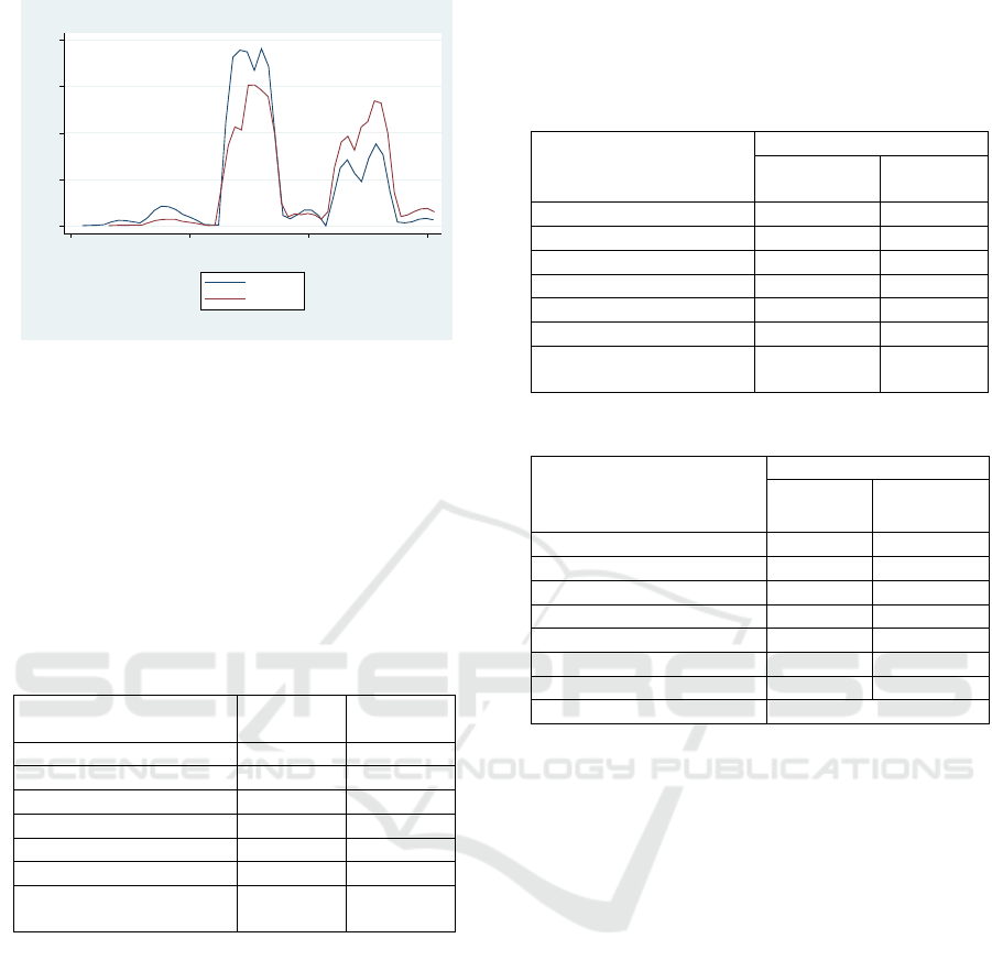
Figure 4: Propensity score distribution and common

support for propensity score estimation.

4.4 Assessing Matching Quality

Table 2 shows that all of the variables have a smaller

bias after matching. It is one of the characteristics of

matching quality. But, there is no clear standard for

determining success in bias standard reduction in the

matching method(Caliendo & Kopeinig, 2008).

Table 2: Standardised Bias from NN Without Replacement

Matching.

Variable

Before

Matchin

After

Matchin

HH Job -11.30 -6.50

Java 10.80 2.70

Wall Material -14.50 -0.30

Floor Material -17.90 0.20

Roof T

e -7.70 0.00

Electricit

7.20 0.00

Water source for

drinking 41.00 0.30

Table 3 presents the p-value of t-test for before

and after matching equations. Before matching all of

control variables (covariates) had a different mean

between the treated household and the untreated

household. After the matching, only two covariates

have an average that does not differ between the two

groups (HH job and Roof type). It indicates that the

model already has a good matching quality.

A joint test for equality of means in all control

variables can be conducted after testing the difference

of control variables means individually. By testing

the Hotelling-test using STATA 15, the result (table

4) shows that the p-value of the F test is smaller than

5%, which is 0.000. It indicates the means of the two

group is not equal. But it shows that there is no large

different between the two group, hence the

conditioning variables are well jointly.

Table 3: Test for Equality of The Mean Before and After

Matching (t-test).

Variable

P-value of t-test

Before

Matching

After

Matching

HH Job 0.000 0.000

Java 0.000 0.054

Wall Material 0.000 0.767

Floor Material 0.000 0.855

Roof Type 0.000 0.000

Electricit

0.000 1.000

Water source for

drinking 0.000 0.856

Table 4: Hotelling-test After Matching.

Covariates

Mean Fo

Program

Recipient

Non-

Recipient

HH Job 0.900 0.932

Java 0.583 0.529

Wall Material 0.014 0.037

Floor Material 0.014 0.043

Roof Type 0.002 0.008

Electricit

0.996 0.990

Water source for drinkin

0.483 0.287

Hotelling p-value 0.000

4.5 Sensitivity Analysis

In this study, the point estimation of Rosenbaum’s

bounds for the p-values with Γ=1 is very close to the

estimation in the propensity score matching analysis.

The estimation effect of NN matching is 0.289 which

is significant at the 1% and the Hodges-Lehman point

estimate is 0.285 significant at the 1%. Table 5 shows

the results of this sensitivity analysis for the impact of

internet access on household expenditure using

Wilcoxon's signed rank test.

Table 5 also shows that for an increase of Γ=0.9,

p-value increases to 0.086 in the upper bound (greater

than 0.05). In this study, a hidden bias or selection

bias of size Γ=1.9 is sufficient to explain the observed

difference in test scores between the treated

household and the control household. Therefore, two

households that have the same covariates and appear

similar could differ in their odds of having the internet

access by as much as a factor of 1.9. Because 1.9 is a

small value, it shows that this study is sensitive to

hidden bias.

0 2 4 6 8

Density

0 .2 .4 .6

psmatch2: Propensity Score

untreated

treated

kernel = epanechnikov, bandwidth = 0.0133

Kernel density estimate

EBIC 2019 - Economics and Business International Conference 2019

546

Table 5: The Rosenbaum Sensitivity Analysis.

p-value of Wilcoxon’s

signed-rank test

Hodges-Lehman

point estimate

Upper

Boun

Lower

Boun

Upper

Boun

Lower

Boun

1 0.000 0.000 0.285 0.285

1.3 0.000 0.000 0.173 0.397

1.6 0.000 0.000 0.085 0.485

1.8 0.000 0.000 0.036 0.535

1.9 0.086 0.000 0.014 0.558

2 0.776 0.000 -0.008 0.579

4.6 The Impact of Internet Access

If the quality of matching is satisfied, then it is

possible to estimate the Average Treatment Effect on

the Treated (ATET) because the control group now

has similar characteristics to the treated group. Table

6 shows an estimate of the impact of internet access

on household expenditure. It shows that there is a

significant impact at 1% by using all of the matching

methods, exclude NN with Replacement.

Table 6: The Impact of Internet Access on Household

Expenditure.

Matching metho

Effect SE t-stat

NN with replacement -0.013 0.393 -0.04

NN without re

lacement 0.289 0.009 29.08

Kernel 0.297 0.009 32.34

Radius Cali

0.295 0.009 31.97

Based on the data distribution, this study

determines the Impact of internet access by using

matching NN without replacement method. The

upper-bound value of Hodges-Lehman Point on the

sensitivity analysis when Γ=1 and the ATT value is

0.28. It indicates that households having internet

access have about 29% higher expenditure than other

households. This is in line with research conducted by

Hong (2007); Colley & Maltby (2008); Khanal &

Mishra (2013); Van Heddeghem et al (2014); and

Zhang et al (2017).

5 CONCLUSIONS

Based on those analyses and results that have been

explained, then the conclusions obtained from this

study are as follows. First, internet access have a

significant impact on increasing household

expenditure. Households having internet access have

about 29% higher expenditure than other households.

Second, this paper can prove that The more poor a

household, the smaller the probability of a household

to have the internet access.

As a result, The government needs to equalize

access to information technology, especially the

internet access. However, the government also needs

to control the freedom of use of information

technology. In addition, households should also use

internet access not only for consumption, but for

investment or for entrepreneurship. Because, this can

encourage an increase in household income and will

further increase economic growth in Indonesia.

REFERENCES

Caliendo, M., & Kopeinig, S. (2008). Some practical

guidance for the implementation of propensity score

matching. Journal of Economic Surveys, 22(1), 31–72.

https://doi.org/10.1111/j.1467-6419.2007.00527.x

Colley, A., & Maltby, J. (2008). Impact of the Internet on

our lives: Male and female personal perspectives.

Computers in Human Behavior, 24(5), 2005–2013.

https://doi.org/10.1016/j.chb.2007.09.002

Gertler, P. J., Martinez, S., Premand, P., Rawlings, L. B., &

Vermeersch, C. M. J. (2011). Impact Evaluation in

Practice (1st ed.). Washington D.C.: World Bank.

https://doi.org/10.1596/978-0-8213-8541-8

Hermawan, H. (2017). CONSUMER ATTITUDES ON

ONLINE SHOPPING. Wacana, 16(1), 136–147.

https://doi.org/https://doi.org/10.32509/wacana.v16i1.

Hong, S. H. (2007). The recent growth of the internet and

changes in household-level demand for entertainment.

Information Economics and Policy, 19(3–4), 304–318.

https://doi.org/10.1016/j.infoecopol.2007.06.004

Irmawati, D. (2011). Utilization of E-Commerce in the

Business World. Business Oration Scientific, 6, 95–

112.

Khanal, A. R., & Mishra, A. K. (2013). Assessing the

impact of internet access on household income and

financial performance of small farms. In Southern

Agricultural Economics Association (SAEA). Retrieved

from

http://ageconsearch.umn.edu/bitstream/143019/1/SAE

A_paper_Aditya_re_18Jan.pdf

OECD. (2019). Household spending (indicator).

https://doi.org/10.1787/b5f46047-en

OJK. (2017). Consumer Education Magazine. Jakarta:

Otorita Jasa Keuangan. Retrieved from www.ojk.go.id

Renteria, C. (2015). How Transformational Mobile

Banking Optimizes Household Expenditures: A Case

Study from Rural Communities in Mexico. Information

Technologies & International Development, 11(3), 39–

54. Retrieved from

http://dev.itidjournal.org/index.php/itid/article/view/14

Rosenbaum, P. R. (2005). Sensitivity Analysis in

Observational Studies Randomization Inference and

The Impact of Internet Access on Household Expenditure using the Matching Method

547

Sensitivity. Encyclopedia of Statistics in Behavioral

Science, 4, 1809–1814.

https://doi.org/10.1002/0470013192.bsa606

Rosenbaum, P. R., & Rubin, D. B. (1983). The Central Role

of the Propensity Score in Observational Studies for

Causal Effects Author ( s ): Paul R . Rosenbaum and

Donald B . Rubin Published by : Oxford University

Press on behalf of Biometrika Trust Stable URL :

http://www.jstor. Biometrika Trust, Oxford University

Press, 70(1), 41–55. Retrieved from

www.jstor.org/stable/2335942

Strauss, J., Witoelar, F., & Sikoki, B. (2016). The Fifth

Wave of the Indonesia Family Life Survey (IFLS5):

Overview and Field Report. Retrieved from WR-

1143/1-NIA/NICHD

Sulistyaningrum, E. (2016). IMPACT EVALUATION OF

THE SCHOOL OPERATIONAL ASSISTANCE

PROGRAM ( BOS ) USING THE MATCHING

METHOD, 31(1), 35–62.

Van Heddeghem, W., Lambert, S., Lannoo, B., Colle, D.,

Pickavet, M., & Demeester, P. (2014). Trends in

worldwide ICT electricity consumption from 2007 to

2012. Computer Communications, 50, 64–76.

https://doi.org/10.1016/j.comcom.2014.02.008

Zhang, A., Lv, J., & Kong, Y. (2017). The Effects of the

Internet and Mobile Services on Urban Household

Expenditures. In 14th International

Telecommunications Society (ITS) Asia-Pacific

Regional Conference. Retrieved from

https://www.econstor.eu/handle/10419/168554

EBIC 2019 - Economics and Business International Conference 2019

548