Market Reaction on Reverse Stock Split Announcement: Empirical
Evidence in Indonesian Stock Market
Edwin Hendra, Theresia Lesmana, and Sasya Sabrina
Accounting Department, Bina Nusantara University, Jl. K.H. Syahdan No. 9, Palmerah, Jakarta, Indonesia
Keywords: Event Study, Reverse Stock Split, Insider Trading
Abstract: This research focuses on reverse stock split announcements. We are trying to examine stock returns behavior
on days prior and following the reverse split announcements. The sample of this study is reverse stock split
events on an Indonesian stock market within the year of 2002-2018. An earlier abnormal stock price
movement before the announcement shows a sign of insider trading existences, and a delayed abnormal stock
price movement following the announcement shows a slow respond of market reaction to particular new
information. We are using cumulative abnormal return (CAR) and cumulative market-adjusted return
(CMAR) to identify the abnormal stock price movement. The results show that there are positive abnormal
returns before the announcement, and then it declines further into negative abnormal returns until post the
announcement. However, when we segregate the sample into four price fractions, we find positive abnormal
returns patterns only appear on two-five thousand rupiahs price fraction. Meanwhile, the other price fraction
categories show declining patterns of negative abnormal returns. Overall, we temporarily suggest that there
are illegal insider trading activities in the Indonesian Stock Market. The immediate market reactions show
that the market is quite efficient, and its responses regarding the reverse stock split event follow the prediction
of the trading range hypothesis.
1 INTRODUCTION
Reverse stock split (reverse split) is a less popular
corporate action relative to a regular (forward) stock
split. The literature has frequently discussed stock
splits across periods and equity markets of countries.
However, the reverse splits have not received many
interests in the academic community since the first
studies by (Fama et al., 1969). The reverse split is a
technical merging number of outstanding shares to
form a smaller number of proportionally higher-
priced shares. Since it is supposed to be purely
cosmetic, theoretically, the reverse split should not
affect future cash flows nor the total value of the
company.
Nevertheless, many studies show mostly negative
market reactions to the stock price following reverse
split announcement (Woolridge and Chambers, 1983;
Lamoureux and Poon, 1987; Peterson and Peterson,
1992; Hwang, 1995; Desai and Jain, 1997).
Following the efficient market hypothesis (Fama,
1969)—the stock price will react to new information.
Thus, the public considers reverse split
announcement as unfavorable information of a firm.
There are three theories—signaling hypothesis,
trading range hypothesis, and liquidity hypothesis,
that may explain what kind of information conveyed
by a stock split announcement, which causes a market
reaction. The signaling hypothesis posits that the
firm’s management wants to convey favorable private
information about the firm’s prospect and therefore
signals undervaluation of the splitting firms (Brennan
and Copeland, 1988; Byun and Rozeff, 2003). The
trading range hypothesis posits that the stock split is
an instant attempt to put the stock price back on an
optimal trading range, which is preferable to investors
(Copeland, 1979; Ikenberry, Rankine, and Stice,
1996; Amihud, Mendelson and Uno, 1999). The
liquidity hypothesis posits that the stock split is an
attempt to increase the liquidity or trading volume,
which in turn increases its split-adjusted price
(Muscarella and Vetsuypens, 1996; Lin, Singh, and
Yu, 2009). For the reverse split cases, trading range
hypothesis is a more suitable explanation, since
usually managers are forced to do a reverse split
rather than do it deliberately (Peterson and Peterson,
1992; Martell and Webb, 2008).
Since stock splits usually convey favorable
information about the firms, thus positive abnormal
154
Hendra, E., Lesmana, T. and Sabrina, S.
Market Reaction on Reverse Stock Split Announcement: Empirical Evidence in Indonesian Stock Market.
DOI: 10.5220/0009200601540161
In Proceedings of the 2nd Economics and Business International Conference (EBIC 2019) - Economics and Business in Industrial Revolution 4.0, pages 154-161
ISBN: 978-989-758-498-5
Copyright
c
 2021 by SCITEPRESS – Science and Technology Publications, Lda. All rights reserved

returns, particularly those coming shortly before a
split’s announcement date, should raise strong
suspicions of insider trading, particularly in nations
with weak regulatory structures (Nguyen, Tran, and
Zeckhauser, 2017). The insider traders may exploit
the leakage of information by buying shares of
splitting firms few days before a split’s
announcement is going public, where it may cause a
sudden increase in the stock prices during that period.
On the contrary, if the insider trader also exists in
reverse split events, then hypothetically, there will be
negative abnormal returns on days before reverse
split’s announcements since the reverse splits are
considered conveying unfavorable information.
Indonesia is one of developing countries with
“adolescence” stock market, yet has excellent growth
potential, and characterized by nonsynchronous
trading, where shares of some listed firms are rarely
traded or not traded at all during a specific period.
Reverse splits in Indonesia stock market usually are
conducted by less big listed firms, which it has
nonsynchronous trading characteristic and rarely
becomes the object of studies. Since Indonesia is one
of the emerging markets, then we can assume that the
Indonesian stock market has no strong regulatory
structure. Thus it may be threatened by some illegal
trading activities.
In this paper, we conduct an event study of reverse
split events in Indonesia stock market. We are trying
to identify the stock price behavior of reverse splitting
firms by analyzing whether there are abnormal
returns during the event window—30 days prior and
30 days post the announcement date. The abnormal
returns before the announcement date may indicate
that there were illegal trading activities. On the other
hand, the abnormal returns post the announcement
date shows a market inefficiency due to the
information delay. Lastly, since reverse splits are
rarely become the object of studies, we hope that our
findings may give a significant contribution to the
reverse split event study literature, particularly in the
emerging market context.
2 LITERATURE REVIEW
Reverse splits are desperate efforts by the firms to
raise their prices high enough to meet the minimum
price required to maintain a listing on the stock
exchange (Martell and Webb, 2008). Sixty-five
percent of the firms with multiple reverse splits end
up being liquidated or delisted. If one reverse split is
a sign of desperation, then multiple reverse splits are
a sign of extreme distress (Crutchley and Swidler,
2015). Reverse split announcements are interpreted as
unfavorable information of the firm because the
manager is considered do not have any other ways to
raise the stock price, thus it results in a negative effect
on the stock returns that happened both on the
announcement date and the effective date of the
reverse splits (Woolridge and Chambers, 1983). The
further researches find negative abnormal returns
since the announcement date of reverse splits, which
continued to accumulate in the short term (Hwang,
1995) and also in the long term (Desai and Jain,
1997).
The signaling hypothesis posits that the abnormal
returns during the stock split show a signal from the
firm’s management that conveys favorable private
information about the firm’s prospects (Brennan and
Copeland, 1988). The increasing stock prices after the
split are followed by increased future dividends that
assume the firms had better performance (Fama et al.,
1969). Splitting firms yield higher earnings growth
than similar, non-splitting firms in the five years
before the split (Lakonishok and Lev, 1987).
Nevertheless, stock splits that are not followed by a
subsequent abnormal return in the long term period
show that the market is efficient (Byun and Rozeff,
2003). In reverse split cases, the signaling hypothesis
is not applicable because it is improbable the manager
would do a deliberate reverse split just to let the
public knows that the price stock is somewhat
overvalued.
The trading range hypothesis suggests that there
is an optimal trading range, and that splits realign
share prices. At the optimal trading range, the stock
will be more frequently traded and get become more
attractive to the investors. Stock splits generally occur
when stocks trade at high prices preceding the split
announcement, which is consistent with the view that
splits are typically used to realign share prices to an
average trading range (Ikenberry, Rankine, and Stice,
1996). Meanwhile, firms do a reverse split is to
increase the marketability of their stocks because the
market will consider a stock with too lower price as a
penny stock, which is speculative and less attractive,
particularly to the institutional investors (Peterson
and Peterson, 1992).
The liquidity hypothesis posits that stock splits
may improve trading continuity, alleviate liquidity
risk and give more benefit to the less liquid stocks
(Lin, Singh and Yu, 2009). A reduction in the
minimum trading unit greatly increases a firm’s base
of individual investors and its stock liquidity, and it is
associated with a significant increase in the stock
price (Amihud, Mendelson and Uno, 1999). Copeland
(1979) shows that there were increasing trading
volume following the stock splits, but not increased
proportionally to its split factor. The increasing
liquidity following the stock split may reduce the
liquidity risk and cause the split-adjusted stock price
to increase substantially. On the contrary, there is a
Market Reaction on Reverse Stock Split Announcement: Empirical Evidence in Indonesian Stock Market
155

possibility the liquidity risk will be decreased
following the reverse split, so that it may cause the
split-adjusted stock price to decrease. Nevertheless, it
would be very unlikely that decreasing liquidity
becomes the ulterior motive behind the reverse split.
Insider trader—the corporate insider who has
more direct access to firm wellbeing, may exploit
their informational advantage about the company to
gain unfair profit from trading activities. In most
nations, it is considered as illegal activities if the trade
was made based on non-public material information.
However, illegal trading is much harder to be studied,
given that perpetrators try to hide their tracks and that
broadly effective detection methods are not available.
Nevertheless, some existing studies have creatively
detected evidence of illegal trades. Bhattacharya,
Daouk, Jorgenson, and Kehr (2000) suggest the
researcher be suspicious of illegal trading activity if
there is nothing happened during the day of the
corporate action announcement and something
happened during the days before the pre-
announcement. Cheng, Nagar, and Rajan (2007)
suggest that the corporate insider has misused the
delay of legal insider trading disclosure to perform
information-based trading.
Nguyen et al. (2017) find that there are incredibly
high abnormal returns and increasing trading volume
before the split announcement, which may indicate
illegal trading activities in the Vietnam stock market.
We suggest that the Indonesian stock market probably
has a weak regulatory structure since it is also one of
the emerging markets as well as Vietnam.
Hypothesis 1: There are earlier abnormal returns
before the reverse split announcement as an
indication of illegal trading activities.
Unlike the regular stock split, successful firms that
receive much attention from the market is unlikely to
conduct a reverse split. On the contrary, it is usually
quite popular among less attractive firms. Thus, we
suggest that the market will react slowly to an
announcement made by this kind of company.
Hypothesis 2: There are delayed abnormal returns
post to the reverse split announcement as an
indication of market inefficiency.
The reverse split theoretically is more in line with the
trading range hypothesis instead of the two others.
The literature mentions that the primary purposes of
the reverse split are fulfilling the listing requirement
(Martell and Webb, 2008) and avoiding the penny
stock label (Peterson and Peterson, 1992). Thus, we
suggest that the market will favor the reverse split
announcement by showing positive abnormal returns.
On the other hand, the literature has documented
empirical evidence of negative market reactions
following reverse split announcements (Woolridge
and Chambers, 1983; Lamoureux and Poon, 1987;
Peterson and Peterson, 1992; Hwang, 1995; Desai
and Jain, 1997).
Hypothesis 3: There are unpredicted abnormal
return patterns following reverse split
announcements.
3 METHOD
We analyze 60 days stock return data—30 days prior
and 30 days post to the reverse split announcement—
as the event window. The sample is stocks listed on
the Indonesia Stock Exchange in the year 2002 to
2018. There were 49 reverse split events during those
years, but due to the limitation of data, we can only
observe 44 split events as the research sample. The
stock split announcement dates are derived from
KSEI’s (Kustodian Sentral Efek Indonesia) official
website. The stock prices and market index are
gathered from the Thomson Reuters Data Stream.
The daily stock return and market return are
calculated using a simple stock return formula, as in
equation (1) and (2).
𝑅


𝑃

𝑃

𝑃



(1)
𝑅


𝐼𝑛𝑑𝑒𝑥

𝐼𝑛𝑑𝑒𝑥

𝐼𝑛𝑑𝑒𝑥


(2)
We were using two kinds of abnormal return
measurements—Cumulative Market Adjusted Return
(CMAR) and Cumulative Abnormal Return (CAR)—
to analyze the market reaction during the event
window as in equation (3) and (4).
𝐶𝑀𝐴𝑅
,
1𝑅

𝑅






1
(3)
𝐶𝐴𝑅
,
𝑅

𝛼

𝛽

𝑅






(4)
We measure the alpha and beta of each stock
using the single index model in equation (5) by
regressing 250 daily returns before the event window.
𝑅

𝛼

𝛽

𝑅

𝑢

(5)
We analyze the univariate test—using SPSS 24
statistic software—for hypothesis testing. We use the
one-sample t-test and Kolmogorov-Smirnov test in
EBIC 2019 - Economics and Business International Conference 2019
156

identifying whether abnormal return and cumulative
abnormal return are significantly different from zero
and not normally distributed during a particular event
day.
4 RESULTS AND DISCUSSION
Table 1 shows the detail of the reverse stock split
announcement sample. The reverse stock split events
most frequently happened during the year of 2002 –
2005 and becoming less frequent in years after, with
the most commonly chosen split factor are between
1:4 and 1:10.
Table 1. Reverse Stock Split Announcement Sample
Year Split Factor
1:2 1:4-
6
1:8-
10
1:15-
25
1:100 Tot
al
02-05 2 4 10 4 1 21
06-10 4 5 1 1 - 11
11-14 - 1 2 1 - 4
15-18 - 2 5 - 1 8
Total 6 12 18 6 2 44
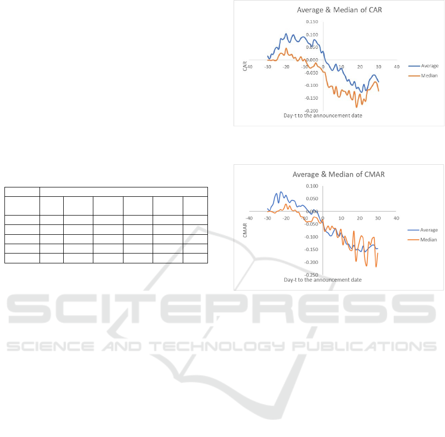
Figure 1 shows the average and median of CAR
of the reverse stock split events. Both graphs show a
similar pattern that the CAR is increasing since day t-
30, and it starts to decline after day t-20. After the
announcements, the CAR is dropping further and
begins to rebound on day t+20. Figure 2 shows the
average and median of CMAR of the reverse stock
split events. The graphs of CMAR tell a similar story,
but it already shows indications of negative abnormal
return before the announcements.
Table 2 and Table 3 show the descriptive statistics
of CAR and CMAR on the event window. We only
use 36 reverse split events on CAR calculation, since
we could not estimate the coefficient regression of the
single index model due to the inactive transaction of
the stocks during the estimation period. One Sample
t-test shows a significantly positive result on CAR
and CMAR on the day t-20. Meanwhile, the
Kolmogorov-Smirnov test shows a significant result
for all day before the announcement for both CAR
and CMAR. On the one hand, the average CAR on
the days before the announcement shows a positive
sign. On the other hand, the median CAR, average
CMAR, and median CMAR have already reversed
the sign to be negative before the announcement day.
Figure 1: Average CAR and Median CAR of Reverse Split
Events
Figure 2: Average CMAR and Median CMAR of Reverse
Split Events
CAR and CMAR show a declining pattern post of
the announcement day. For the CAR, the one-sample
t-tests do not show any significant result. Meanwhile,
the Kolmogorov-Smirnov tests show a significant
result at least for ten days post to the announcement
day. On the contrary, the one-sample t-tests show a
longer-term significance on CMAR, while the
Kolmogorov-Smirnov tests provide similar results in
comparison with CAR. According to these findings,
on the averages, our results support the first
hypothesis rather than the second hypothesis.
Just like a regular stock split, a reverse split is also
not just a purely cosmetic. These findings provide
evidence that the reverse splits convey specific
information. Our results in line with the previous
literature (Woolridge and Chambers, 1983;
Lamoureux and Poon, 1987; Peterson and Peterson,
1992; Hwang, 1995; Desai and Jain, 1997) that the
market reacts negatively on the stock prices following
the reverse split announcement. These reactions are
immediate following the announcement. Thus, we
may suggest that the Indonesian stock market is quite
efficient regarding this matter.
Market Reaction on Reverse Stock Split Announcement: Empirical Evidence in Indonesian Stock Market
157

Table 2: Cross-sectional Average and Median of CAR and
CMAR Between Day -30 and Day 0
Day-
t
CAR CMAR
Average Median Average Median
-30 0.016 0.000
***
0.012 -0.002
***
-29 0.005 0.000
***
0.003 0.001
***
-28 0.024 -0.001
***
0.018 -0.001
***
-27 0.023 0.001
***
0.030 -0.003
***
-26 0.044 -0.002
***
0.060 -0.006
***
-25 0.051 0.001
***
0.071 -0.001
***
-24 0.043 0.017
***
0.034 0.002
***
-23 0.084 0.027
***
0.076 0.008
***
-22 0.081 0.025
***
0.071 0.004
***
-21 0.088 0.020
***
0.053 0.013
***
-20 0.104
*
0.047
***
0.064
*
0.029
***
-19 0.080 0.024
***
0.046 0.009
***
-18 0.070 0.019
***
0.036 0.022
***
-17 0.089 0.022
***
0.044 0.008
***
-16 0.100 0.008
***
0.044 0.002
***
-15 0.082 0.010
***
0.039 0.006
***
-14 0.074 -0.003
***
0.019 -0.003
***
-13 0.074 0.002
***
0.022 -0.004
***
-12 0.087 0.013
***
0.021 -0.020
***
-11 0.091 -0.003
***
0.025 -0.021
***
-10 0.089 0.003
***
0.021 -0.031
***
-9 0.079 -0.010
***
0.012 -0.040
***
-8 0.067 -0.024
***
0.004 -0.040
***
-7 0.063 -0.032
***
-0.004 -0.039
***
-6 0.054 -0.028
***
-0.010 -0.038
***
-5 0.079 -0.024
***
0.008 -0.023
***
-4 0.076 -0.011
***
0.002 -0.023
***
-3 0.064 -0.024
***
-0.002 -0.027
***
-2 0.057 -0.028
***
-0.020 -0.042
***
-1 0.029 -0.035
***
-0.037 -0.046
***
0 0.034 -0.047
***
-0.043 -0.033
***
Notes: *, **, and *** denote statistically different than zero
at 10%, 5%, and 1% levels respectively for one-sample t-
test (on the average column) and one-sample Kolmogorov-
Smirnov test (on the median column)
Figure 3 and Figure 4 show the average and the
median of CAR, on various expected stock price
faction after the reverse split is executed—day 0 price
times the split factor. We arbitrarily determine the
nominal price classification just based on the current
BEI’s price fraction for regular trading. The nominal
price fraction of two thousand until five thousand
rupiahs has a positive value in the average and the
median of CAR for the whole event window periods.
Meanwhile, the other price fractions show a negative
value with a declining pattern, whereas the price
fraction above five thousand rupiahs has the most
extreme declining.
Table 3: Cross-sectional Average and Median of CAR and
CMAR Between Day 0 and Day +30
Day-
t
CAR CMAR
Average Median Average Median
0 0.034 -0.047
***
-0.043 -0.033
***
1 0.002 -0.049
***
-0.067 -0.078
***
2 -0.011 -0.083
***
-0.080
*
-0.069
**
3 -0.017 -0.107
***
-0.085
**
-0.057
***
4 -0.032 -0.102
***
-0.095
**
-0.072
***
5 -0.041 -0.104
**
-0.093
**
-0.058
***
6 -0.029 -0.133
**
-0.078 -0.067
***
7 -0.016 -0.103
**
-0.066 -0.067
**
8 -0.042 -0.141
*
-0.087
*
-0.102
***
9 -0.038 -0.144
*
-0.097
**
-0.093
*
10 -0.033 -0.118
**
-0.084
*
-0.070
**
11 -0.051 -0.122 -0.099
*
-0.132
**
12 -0.064 -0.124 -0.109
**
-0.097
**
13 -0.082 -0.137 -0.128
**
-0.112
14 -0.077 -0.120 -0.127
**
-0.136
15 -0.095 -0.147 -0.140
***
-0.152
16 -0.098 -0.155 -0.145
***
-0.153
17 -0.084 -0.123 -0.133
***
-0.078
**
18 -0.111 -0.184 -0.150
***
-0.194
19 -0.107 -0.155 -0.147
***
-0.153
20 -0.120 -0.133 -0.153
***
-0.119
21 -0.126 -0.173 -0.157
***
-0.095
22 -0.095 -0.153 -0.135
**
-0.106
23 -0.119 -0.161 -0.158
***
-0.188
24 -0.110 -0.118 -0.152
***
-0.213
25 -0.080 -0.117 -0.143
**
-0.120
26 -0.070 -0.108 -0.138
**
-0.132
**
27 -0.059 -0.096 -0.132
**
-0.107
28 -0.059 -0.085 -0.133
**
-0.102
29 -0.072 -0.091 -0.145
**
-0.217
30 -0.086 -0.121 -0.145
**
-0.164
Notes: *, **, and *** denote statistically different than zero
at 10%, 5%, and 1% levels respectively for one-sample t-
test (on the average column) and one-sample Kolmogorov-
Smirnov test (on the median column)
Table 4 and Table 5 show a cross-sectional
average of CAR on each price fraction category
during the event window. One-sample t-test shows a
weakly significantly positive CAR on a few days
before the announcement for the two-five thousand
rupiahs price fraction. On the contrary, there is a
significantly negative CAR on days post the
announcement for the above five thousand rupiahs
price fraction.
Table 6 and Table 7 show a cross-sectional
median of CAR on each price fraction category
during the event window. Kolmogorov-Smirnov test
shows significant results only for the days before the
announcement. The results are entirely consistent,
that positively significant CAR is found on two-five
thousand rupiahs price fraction, while negatively
significant CAR is found on the other price fractions.
Thus, overall, our findings support the third
hypothesis.
EBIC 2019 - Economics and Business International Conference 2019
158

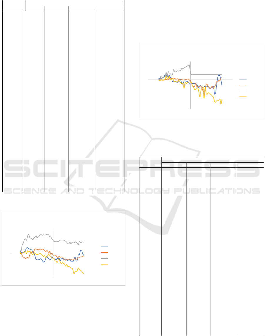
Table 4: Cross-sectional Average of CAR on Expected
Stock Price Fraction Between Day -30 and Day 0
Day-t
CAR
<500 500-1999 2000-4999 >5000
-30 0.047 -0.017 0.048 0.008
-29 0.008 -0.015 0.047 -0.014
-28 0.005 -0.057
*
0.175 -0.007
-27 0.000 -0.089 0.209 0.002
-26 0.026 -0.098
*
0.282 0.007
-25 0.055 -0.121 0.298 0.030
-24 0.102
*
-0.106 0.265 -0.018
-23 0.106
*
-0.095 0.349 0.044
-22 0.091
*
-0.110 0.395
*
0.013
-21 0.078 -0.047 0.327
*
0.033
-20 0.072 0.019 0.312 0.033
-19 0.059 0.005 0.298 -0.025
-18 0.018 0.023 0.276 -0.039
-17 -0.002 0.035 0.318 -0.006
-16 -0.067 0.088 0.334
*
-0.007
-15 -0.144 0.075 0.363
*
-0.038
-14 -0.132 0.078 0.319
*
-0.040
-13 -0.140 0.056 0.346
*
-0.030
-12 -0.150 0.083 0.364
*
-0.028
-11 -0.125 0.058 0.382
*
-0.011
-10 -0.132 0.074 0.386
*
-0.038
-9 -0.165 0.082 0.370
*
-0.053
-8 -0.196 0.070 0.383
*
-0.080
-7 -0.189 0.046 0.375
*
-0.060
-6 -0.131 0.021 0.376
*
-0.103
-5 -0.076 0.048 0.392
*
-0.087
-4 -0.105 0.037 0.381
*
-0.056
-3 -0.121 -0.008 0.383
*
-0.037
-2 -0.139 0.035 0.334 -0.058
-1 -0.138 -0.034 0.341 -0.086
0 -0.079 -0.002 0.297 -0.105
Notes: *, **, and *** denote statistically different than zero
at 10%, 5%, and 1% levels respectively for one sample t-
test.
Figure 3: Average CAR of Each Expected Stock Price
Fractions
Our findings are also in line with the trading range
hypothesis and liquidity hypothesis. We temporarily
suggest that the nominal price in between two
thousand and five thousand rupiahs is the optimal
trading range. Thus the market reacts positively to the
reverse split attempts to put the nominal stock price
in that ranges (Ikenberry, Rankine, and Stice, 1996).
On the other hand, within the context of reverse split,
we temporarily suggest that the market still considers
the stock traded below two thousand rupiahs as a
penny stock (Peterson and Peterson, 1992) and the
stock traded above five thousand rupiahs will become
further less liquid (Amihud, Mendelson and Uno,
1999; Lin, Singh and Yu, 2009). Therefore, the
market reacts negatively to these categories of the
reverse split.
Figure 4: Median CAR of Each Expected Stock Price
Fractions
Table 5: Cross-sectional Average of CAR on Expected
Stock Price Fraction Between Day 0 and Day +30
Day-t
CAR
<500 500-1999 2000-4999 >5000
0 0.047 -0.017 0.048 0.008
1 0.008 -0.015 0.047 -0.014
2 0.005 -0.057 0.175 -0.007
3 0.000 -0.089 0.209 0.002
*
4 0.026 -0.098 0.282 0.007
*
5 0.055 -0.121 0.298 0.030
*
6 0.102 -0.106 0.265 -0.018
*
7 0.106 -0.095 0.349 0.044
*
8 0.091 -0.110 0.395 0.013
**
9 0.078 -0.047 0.327 0.033
**
10 0.072 0.019 0.312 0.033
**
11 0.059 0.005 0.298 -0.025
*
12 0.018 0.023 0.276 -0.039
*
13 -0.002 0.035 0.318 -0.006
**
14 -0.067 0.088 0.334 -0.007
*
15 -0.144 0.075 0.363 -0.038
**
16 -0.132 0.078 0.319 -0.040
**
17 -0.140 0.056 0.346 -0.030
**
18 -0.150 0.083 0.364 -0.028
**
19 -0.125 0.058 0.382 -0.011
**
20 -0.132 0.074 0.386 -0.038
**
21 -0.165 0.082 0.370 -0.053
**
22 -0.196 0.070 0.383 -0.080
**
23 -0.189 0.046 0.375 -0.060
**
24 -0.131 0.021 0.376 -0.103
**
25 -0.076 0.048 0.392 -0.087
**
26 -0.105 0.037 0.381 -0.056
***
27 -0.121 -0.008 0.383 -0.037
**
28 -0.139 0.035 0.334 -0.058
**
29 -0.138 -0.034 0.341 -0.086
**
30 -0.079 -0.002 0.297 -0.105
**
Notes: *, **, and *** denote statistically different than zero
at 10%, 5%, and 1% levels respectively for one sample t-
test.
‐0.500
‐0.400
‐0.300
‐0.200
‐0.100
0.000
0.100
0.200
0.300
0.400
0.500
‐40‐30‐20‐100 10203040
CAR
Day‐ttotheannocementdate
AverageCARofEachExpectedStockPrice
Fractions
<500
500‐1999
2000‐4999
>5000
‐0.5
‐0.4
‐0.3
‐0.2
‐0.1
0
0.1
0.2
0.3
‐40‐30‐20‐10 0 10 20 30 40
CAR
Day‐ttotheannocementdate
MedianCARonofEachExpectedStockPrice
Fractions
≤500
500‐1999
2000‐4999
≥5000
Market Reaction on Reverse Stock Split Announcement: Empirical Evidence in Indonesian Stock Market
159

Table 6: Cross-sectional Median of CAR on Expected
Stock Price Fraction Between Day -30 and Day 0
Day-t
CAR
<500 500-1999 2000-4999 >5000
-30
0.013
**
-0.001
***
0.001
***
-0.013
**
-29
0.019 -0.002
***
0.001
***
-0.019
-28
0.017
**
-0.010
**
0.057
***
-0.013
-27
0.020
**
-0.009
***
0.050
***
0.000
-26
0.028 -0.010
**
0.018
***
-0.017
*
-25
0.033 -0.012
***
0.048
***
-0.001
**
-24
0.084 -0.003
***
0.039
***
-0.004
*
-23
0.073 0.004
***
0.119
**
0.057
-22
0.056 -0.003
**
0.048
***
0.009
-21
0.043 -0.007 0.134
**
0.021
-20
0.076 0.021 0.092
**
0.058
-19
0.036 0.024 0.097
**
-0.001
***
-18
0.015 0.017 0.074
*
-0.005
-17
-0.034 0.021
***
0.080
**
0.021
-16
-0.040 0.008
***
0.166 -0.021
*
-15
-0.046 0.024
**
0.138 -0.037
-14
-0.033
***
0.005
**
0.126 -0.029
-13
-0.048 0.007 0.138
*
-0.027
-12
-0.049 0.013
**
0.149 -0.032
-11
-0.034
**
-0.001
*
0.140 -0.009
**
-10
0.011
*
-0.005
*
0.148 -0.045
-9
-0.018
*
-0.006
**
0.160 -0.055
-8
-0.078
*
-0.003
*
0.192 -0.078
**
-7
-0.074
*
-0.009 0.183 -0.069
**
-6
-0.031 -0.007
**
0.195 -0.147
-5
-0.024 -0.004 0.205 -0.050
-4
-0.032 0.000 0.215 -0.072
-3
-0.030 0.005 0.226 -0.056
-2
-0.042
*
0.010 0.236 -0.042
-1
-0.065 -0.009 0.247 -0.044
0
-0.060 -0.019 0.121 -0.049
Notes: *, **, and *** denote statistically different than zero
at 10%, 5%, and 1% levels respectively for Kolmogorov-
Smirnov test.
5 CONCLUSIONS
The reverse split announcement events are responded
well in the Indonesian stock market, even though it
was a less popular corporate event conducted by less
popular firms. It shows that the Indonesian stock
market is quite efficient. The declining pattern of
cumulative abnormal returns shows that the market
sees the reverse split events as a negative signal, and
we find our results are consistent with the previous
literature. The early market reactions on several days
before the announcement may indicate the existence
of illegal insider trading activities. These reactions
may be various, but we find that it may depend on the
expected stock price after the reverse split is
Table 7: Cross-sectional Median of CAR on Expected
Stock Price Fraction Between Day -30 and Day 0
Day-t
CAR
<500 500-1999 2000-4999 >5000
0
-0.060
-0.019 0.121 -0.049
1
-0.070 -0.056 0.083 -0.046
2
-0.068 -0.112 0.083 -0.109
3
-0.070 -0.118 0.083 -0.128
4
-0.071 -0.123 0.083 -0.172
5
-0.067 -0.062 0.083 -0.166
6
-0.083 -0.117 0.083 -0.140
7
-0.102 -0.117 0.083 -0.143
8
-0.141 -0.122 0.083 -0.203
9
-0.104 -0.108 0.083 -0.296
10
-0.109 -0.116 0.083 -0.193
11
-0.136 -0.139 0.083 -0.139
12
-0.134 -0.196 0.083 -0.130
13
-0.127 -0.204 0.083 -0.319
14
-0.116 -0.201 0.083 -0.122
15
-0.127 -0.080 0.083 -0.243
16
-0.120 -0.083 0.083 -0.249
17
-0.118 -0.123 0.083 -0.224
18
-0.147 -0.136 0.083 -0.240
19
-0.153 -0.150 0.083 -0.248
20
-0.140 -0.125 0.083 -0.263
21
-0.146 -0.116 0.083 -0.284
22
-0.119 -0.153 0.083 -0.305
23
-0.250 -0.111 0.083 -0.379
24
-0.228 -0.094 0.083 -0.383
25
-0.092 -0.036 0.083 -0.360
26
0.032 -0.041 0.083 -0.360
27
0.075 -0.013 0.083 -0.349
28
0.059 -0.025 0.083 -0.331
29
-0.010 0.027 0.083 -0.416
30
-0.099 0.027 0.083 -0.339
Notes: *, **, and *** denote statistically different than zero
at 10%, 5%, and 1% levels respectively for Kolmogorov-
Smirnov test.
executed. The positive abnormal returns average on
certain price fraction, particularly between two
thousand and five thousand rupiahs, show that there
is an optimal trading price as predicted by the trading-
range hypothesis. Meanwhile, the declining pattern of
negative abnormal returns on the above five thousand
rupiahs price fraction is consistent with the liquidity
hypothesis’ prediction.
ACKNOWLEDGMENTS
The authors gratefully acknowledge that the present
research is assisted by Tita Nuvita from Institut Bisnis
Nusantara and Arfan Wiraguna from Prasetya Mulya
University in the data processing and supported
EBIC 2019 - Economics and Business International Conference 2019
160

financially by the 2019 research grant of Bina
Nusantara University.
REFERENCES
Amihud, Y., Mendelson, H. and Uno, J. (1999) ‘Number of
shareholders and stock prices: Evidence from Japan’,
Journal of Finance, 54(3), pp. 1169–1184.
Bhattacharya, U. et al. (2000) ‘When an event is not an
event: The curious case of an emerging market’,
Journal of Financial Economics, 55(1), pp. 69–101.
Brennan, M. J. and Copeland, T. E. (1988) ‘Stock splits,
stock prices, and transaction costs’, Journal of
Financial Economics, pp. 83–101.
Byun, J. and Rozeff, M. S. (2003) ‘Long-Run performance
after stock splits: 1927 to 1996’, Journal of Finance,
58(3), pp. 1063–1085.
Cheng, S., Nagar, V. and Rajan, M. V. (2007) ‘Insider
trades and private information: The special case of
delayed-disclosure trades’, Review of Financial
Studies, 20(6), pp. 1833–1864.
Copeland, T. E. (1979) ‘Liquidity changes following stock
split’, Journal of Finance, 34(1), pp. 115–141.
Crutchley, C. E. and Swidler, S. (2015) ‘Multiple reverse
stock splits (investors beware!)’, Journal of Economics
and Finance, 39(2), pp. 357–369.
Desai, H. and Jain, P. C. (1997) ‘Long‐run common stock
returns following stock splits and reverse splits’, The
Journal of Business, 70(3), pp. 409–433.
Fama, E. F. (1969) ‘Efficient capital markets: A review of
theory and empirical work’, Journal of Finance, 25(2),
pp. 383–417.
Fama, E. F. et al. (1969) ‘The Adjustment of Stock Prices
to New Information’, International Economic Review,
10(1), pp. 1–21.
Hwang, C. Y. (1995) ‘Microstructure and reverse stock
splits’, Review of Quantitative Finance and
Accounting, 5(2), pp. 169–177.
Ikenberry, D. L., Rankine, G. and Stice, E. K. (1996) ‘What
do stock splits realy signal’, Journal of Financial and
Quantitative Analysis, 31(3), pp. 357–375.
Lakonishok, J. and Lev, B. (1987) ‘Stock splits and stock
dividends: Why, who, and when’, Journal of Finance,
42(4), pp. 913–932.
Lamoureux, C. G. and Poon, P. (1987) ‘The market reaction
to stock splits’, Journal of Finance, 42(5), pp. 1347–
1370.
Lin, J. C., Singh, A. K. and Yu, W. (2009) ‘Stock splits,
trading continuity, and the cost of equity capital’,
Journal of Financial Economics, 93(3), pp. 474–489.
Martell, T. F. and Webb, G. P. (2008) ‘The performance of
stocks that are reverse split’, Review of Quantitative
Finance and Accounting, 30(3), pp. 253–279.
Muscarella, C. J. and Vetsuypens, M. R. (1996) ‘Stock
splits: Signaling or liquidity? The case of ADR “solo-
splits”’, Journal of Financial Economics, 42(1), pp. 3–
26.
Nguyen, V., Tran, A. and Zeckhauser, R. (2017) ‘Stock
splits to profit insider trading: Lessons from an
emerging market’, Journal of International Money and
Finance, 74(1), pp. 69–87.
Peterson, D. R. and Peterson, P. P. (1992) ‘A further
understanding of stock distributions: The case of
reverse stock splits’, Journal of Financial Research,
15(3), pp. 189–205.
Woolridge, J. R. and Chambers, D. R. (1983) ‘Reverse
splits and shareholder wealth’, Financial Management,
12(3), pp. 5–15.
Market Reaction on Reverse Stock Split Announcement: Empirical Evidence in Indonesian Stock Market
161