Analysis of Economy in the Improvement of Oil Production using

Hydraulic Pumping Unit in X Field

Muhammad Ariyon, Novia Rita and Tribowo Setiawan

Department of Petroleum Engineering, Universitas Islam Riau, Pekanbaru, Indonesia

Keywords:

Hydraulic Pumping Unit, Eﬁsiensi Volumetris NPV, IRR, POT, DPI.

Abstract:

The wells of X ﬁelds are vertical wells with installed pumps being the Hydraulic Pumping Unit. The wells can

still be optimized by improving the performance of N and SL by trial and error method. Based on optimation

analysis result at well BM 1 by changing SPM and SL parameters on pump which installed with N 6 SPM and

SL 100 inch got Qt equal to 144 bfpd, then converted to N 7 SPM and SL 100 inch so that there increase of

Qt become equal to 199 bfpd And pump efﬁciency from 67% to 80%. While in the well BM 2 by changing

the parameters of SPM and SL on pumps installed with N 8 SPM and SL 100 inch obtained Qt of 284 bfpd,

then converted to N 10 SPM and SL 110 inch so that there is an increase of Qt to equal to 583 bfpd pump

efﬁciency of 65% to 90%. In the economic analysis with Production Sharing Contract system can be known

with non-capital investment of MMUS $ 0.150, obtained NPV contractor MUS $ 451.07, IRR> MARR,POT

< 1 year and DPI 4.00.

1 INTRODUCTION

The oil production process by using the Hydraulic

Pumping Unit (HPU) on the X ﬁeld does not always

work optimally so that the oil ﬂow rate cannot be fully

produced optimally and makes the economic results

of the production not obtained. According to the

discussion of (Brown, 1984), the ability of a well to

produce can be known by calculating the productivity

of wells using IPR curves based on actual data in the

ﬁeld. Optimization of the production rate can be done

by conducting a trial and error method for changes in

Stroke Per Minute (SPM) and Stroke Length (SL) of

the pump.

The purpose of this study is to evaluate the

production performance of the installed hydraulic

pumping unit, to optimize the HPU to increase the

rate of production (Babbitt and Vincent, 2012; Beard,

2013; Pickford and Morris, 1989). Analyze the

economy of the HPU after obtaining a new production

rate.

2 METHOD

This research was conducted at X Field.

Administratively, X Field is located in Siak Sri

Indrapura Regency, Riau Province, Indonesia.

Geologically, the X ﬁeld is located in the Central

Sumatra Basin. X Field has a very large oil content

and shallow well depth where Original Oil In Place

is 101.4 MMSTB with Recovery Factor 47.48%.The

well type on X Field is vertical well and directional

well. The wells to be examined in this research are

BM # 1 and BM # 2 Wells.

Figure 1: Research sites

The research method used is ﬁeld research or

this research use data from oil ﬁeld. The data

102

Ariyon, M., Rita, N. and Setiawan, T.

Analysis of Economy in the Improvement of Oil Production using Hydraulic Pumping Unit in X Field.

DOI: 10.5220/0009129401020108

In Proceedings of the Second International Conference on Science, Engineering and Technology (ICoSET 2019), pages 102-108

ISBN: 978-989-758-463-3

used are secondary data provided by ﬁeld guides,

expert opinions, principles and theories of guaranteed

literature.

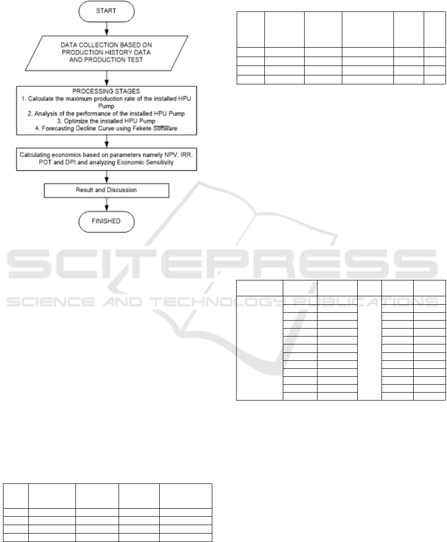
Figure 2: Research ﬂowchart.

3 RESULT AND DISCUSSION

3.1 Determination of Well Performance

and Maximum Flow Rate (Qmax)

with Vogel Method

In knowing whether 4 wells in the X ﬁeld can be

optimized, it is necessary to know the maximum

ﬂow rate (Qmax) in 4 wells with the HPU installed.

The method used in determining Qmax is the Vogel

method because the reservoir ﬂuid ﬂowing in the well

is 2 phase and 50-80% water cut (WC) (Chase and

Shaver, 2009; Ogunleye, 2012).

Table 1: The calculation results determine Sg Fluid,

Gradient Fluid, Pr and Pwf.

WELL Speciﬁc

gravity ﬂuid

(SgFluid).

Gradient

ﬂuid (Gf)

Reservoir

pressure

(Pr)

Bottom well

ﬂow pressure

(Pwf)

BM 1 0.92 0.400 146 78

BM 2 0.97 0.420 55 41

BM 3 0.977 0.423 84 33

BM 4 0.94 0.407 50.8 5.6

After obtaining Sg ﬂuid, Gradient ﬂuid, Pr and

Pwf in table 1, the calculation of the vogel method is

carried out to obtain the maximum ﬂow rate (Qmax),

the following results are obtained.

Table 2: Maximum ﬂow rate in the well on the use of the

installed HPU.

WELL Fluid

Flow

Rate (Qt)

BBL/D

Opt

Flow

Rate of

oil (Qo)

Max Flow

Rate (Qmax)

BBL/D

WC % PI

BM 1 144 65 216 50 2.10

BM 2 284 57 696 80 1.94

BM 3 55 8 69 85 1.07

BM 4 88 30 90 69 1.80

Based on production table 2, it can be seen that

from the 4 wells it has a ﬂuid ﬂow rate (Qt) which has

approached Qmax, that is BM3 and BM5 wells while

BM4 wells have reached the economic limit. For this

reason, only 2 wells can be researched to optimize and

analyze the economics of BM1 and BM2 wells.

After ﬁnding out which wells to be optimized,

the BM1 and BM2 wells then need to use the Inﬂow

Performance Relationship curve to describe changes

in the price of the well bottom ﬂow pressure (Pwf)

versus the ﬂow rate (Q) produced. Then the results

of changes in the bottom well pressure are obtained

from the ﬂow rate in table 3.

Table 3: Results of changes in bottom well ﬂow pressure to

ﬂow rate.

Well Pwf (psi)

Well

Pwf Q

(Bfpd) (psi) (bfpd)

146 0

BM 2

55 0

125 52 50 109

105 95 45 209

95 114 40 300

85 132 35 381

75 148 30 454

BM 1 65 162 25 517

55 175 20 571

45 186 15 616

30 199 10 651

15 209 8 663

10 212 5 678

0 216 0 696

HPU performance known by making IPR curves

using the vogel method which aims to determine the

maximum pump ﬂow rate, because in ﬁeld X has a

two-phase ﬂow, where (Wiggins et al., 1996) states

the vogel method is usually used to determine the

maximum ﬂow rate of two ﬂuid phases.

After obtaining Pwf against Q by assuming Pwf

in table 3, the IPR curve (Inﬂow Performance

Relationship) plot can be performed on BM1 and BM

2 wells.

After knowing the Qmax and Pwf assumptions

towards each Q, then the next step is to know the

volumetric efﬁciency of the HPU installed in wells

BM1 and BM2.

Analysis of Economy in the Improvement of Oil Production using Hydraulic Pumping Unit in X Field

103

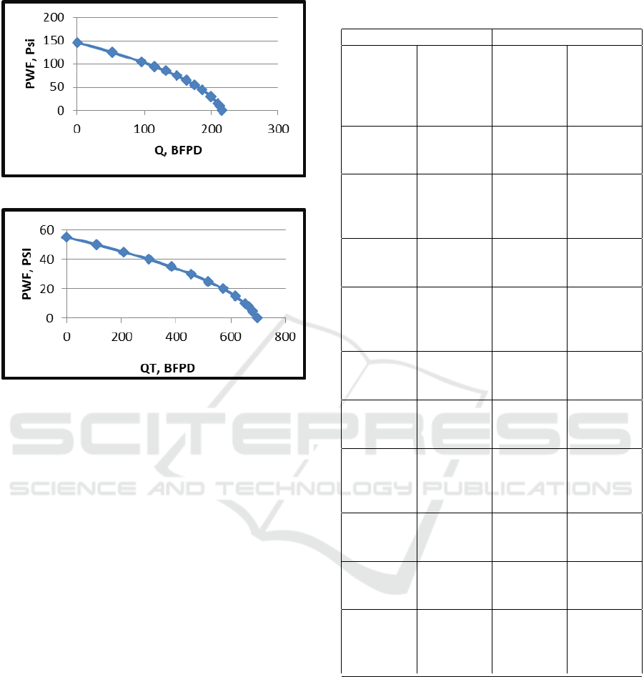
Figure 3: Pwf vs Q IPR curve in BM 1 well.

Figure 4: Pwf vs Q IPR curve in BM 2 well.

3.2 Volumetric Efﬁciency of HPU

Installed in BM1 and BM2 Wells

The procedure in determining the design of the HPU

pump uses the (Jennings et al., 1989) procedure where

the author determines the Pump Depth (L) price of

Plunger area (Ap), rod area (Ar), tubing area (Ar),

plunger constant (K) and rod weight (Wr) and the

price of the pump speed (N). In BM1 and BM2 wells,

the ﬂuid ﬂow lane (Qt) is obtained, namely BM1 wells

with 144 BFPD and BM2 with 284 BFPD.

Pump efﬁciency is performed to determine the

optimal pump performance in BM1 and BM2 wells

or not by looking at parameters such as Pump Size /

Plunger diameter (Dp), Pump speed (N, SPM), Pump

step length (SL, In), Acceleration factor (a), Plunger

over travel (ep), Tubing (et) extension, Rod string (er),

Effective plunger stroke (Sp), Pump constant (K),

Pump capacity (V) and Pump volumetric efﬁciency

(Ev) (Cui et al., 2014; Wang et al., 1995; Ye et al.,

2017), then the results in Table 4 are obtained.

Based on Table 4, it can be analyzed that BM1

wells with the use of 6 SPM (Stroke per minute) and

100 SL (Stroke length) and the use of 1.75 in. Plunger

diameter obtained 213 bfpd pump capacity, while Qt

in BM1 wells was 144 bfpd, volumetric efﬁciency

was obtained the pump is 67.40% While for BM2

wells with the use of 8 SPM (Stroke per minute)

Table 4: Results of pump volumetric efﬁciency installed in

BM 1 and BM 2 wells.

WELL BM1 WELL BM2

Pump

Size /

diameter

plunger

1.75

Pump

Size /

diameter

plunger

2.25

(dp, In) (dp, In)

Pump

Speed

Pump

Speed

(N, SPM) (N, SPM)

Pump

Step

length

100

Pump

Step

length

100

(SL, In) (SL, In)

Acceleratio

n factor

0.05

Acceleratio

n factor

0.09

(a) (a)

Plunger

Over

Travel

(ep, In)

0.02 Plunger

Over

Travel

(ep, In)

0.06

Extention

of Tubing

(et, In)

0.04 Extention

of Tubing

(et, In)

0.09

Rod

String

0.18

Rod

String

0.40

(er, In) (er, In)

Effectif

Plunger

99.80

Effectif

Plunger

99.58

Stroke Stroke

(Sp, In) (Sp, In)

Pump

constant

0.36

Pump

constant

0.59

(K) (K)

Pump

Capacity

213.40

Pump

Capacity

469.80

(V, Bfpd) (V, Bfpd)

Volumetric

Pump

Efﬁciency

(Ev, %)

67.40 Volumetric

Pump

Efﬁciency

(Ev, %)

60.45

and 100 SL (Stroke length) and the use of plunger

diameter of 2.25 in, the pump capacity of 469 bfpd

was obtained, while Qt in BM2 wells was 284 bfpd,

the pump obtained a volumetric efﬁciency of 60%.

Based on the parameters in Table 4 and the

Qmax in 2 wells is quite large, the researcher tried

to do optimization by changing the SPM and SL

parameters in the hope of increasing Qt and the

volumetric efﬁciency of the installed pump becoming

more optimal than previously installed.

ICoSET 2019 - The Second International Conference on Science, Engineering and Technology

104

3.3 Optimization of BM1 and BM 2

Wells

Optimization was carried out to increase the

production ﬂow rate in both wells using the trial

and error method. the concept of trial and error

is to change the parameters of SPM and SL on

the installed pump in the hope of increasing the

volumetric efﬁciency of the pump as well as the

ﬂuid ﬂow rate in wells BM1 and BM2. Next is the

efﬁciency of the pump installed before optimization.

Table 5: The results of pump efﬁciency are installed before

optimization.

Well N (SPM)

Qt (BFPD)

Ev WC

(in) (%) (%)

6 100 144 67.4 50

8 100 284 60.4 80

After that, optimization is done by changing the

parameters of SPM and SL using the trial and error

method. Then, it is obtained in table 6 below

Table 6: The results of installed pump efﬁciency after

optimization.

Well N (SPM)

Qt (BFPD)

Ev WC

(in) (%) (%)

7 100 199 80 50

10 110 583 90.4 80

Based on the results of the optimization in Table

6 in BM1 wells by changing the SPM and SL

parameters on the installed pumps with N 6 SPM and

SL 100 in, Qt is 144 bfpd, then converted to N 7 SPM

and SL 100, in this case, there is an increase in Qt

to 199 bfpd and pump efﬁciency from 67% to 80%,

While the results of the optimization in table 6 in the

BM2 well by changing the SPM and SL parameters

on the installed pump with N 8 SPM and SL 100 in, Qt

is 284 bfpd, then converted to N 10 SPM and SL 110,

there is an increase in Qt to 583 bfpd pump efﬁciency

from 65% to 90%.

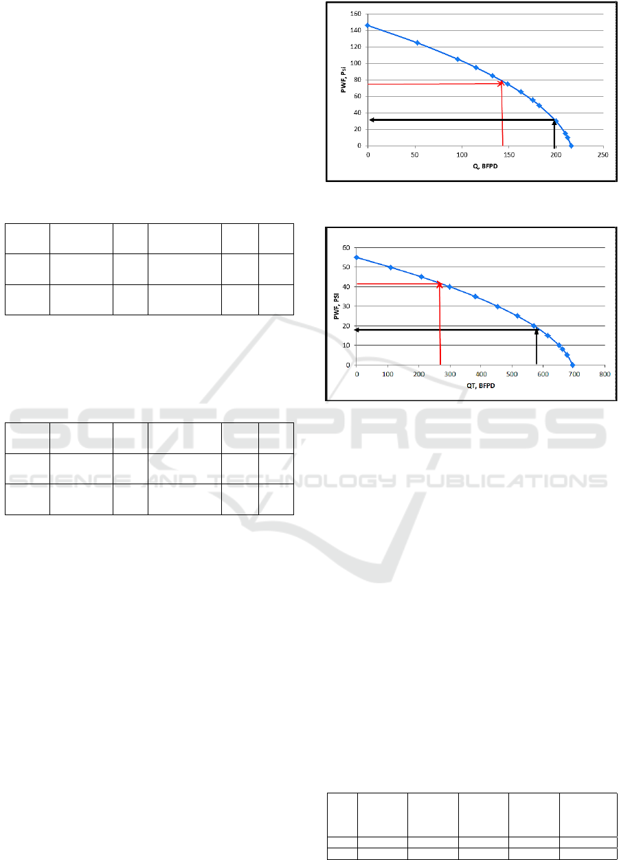
After obtaining the optimum production ﬂow rate,

to determine the bottom well ﬂow pressure (Pwf) in

BM1 and BM2 wells is by plotting the production

ﬂow rate on the IPR curve in each well, the results

are shown in the ﬁgures 5 and 6.

Based on the results of plotting the IPR curves in

Figures 3 and 4 to determine the bottom well ﬂow

pressure (Pwf) with the optimal production ﬂow (Qt)

the results in table 7 on well BM1 with Qt 182 bfpd

Figure 5: IPR curve determination of Pwf against Qt before

and after optimization in BM 1 wells.

Figure 6: IPR curve determination of Pwf against Qt before

and after optimization in BM 2 wells.

obtained pwf 30 psi while the BM2 wells with Qt

583 bfpd obtained pwf 19 psi. Based on the results

of increasing production ﬂow rates in BM1 and BM2

wells, the next step is to forecast with Decline Curve

to ﬁnd out when the production performance will be

in the future.

3.4 Decline Curve Analysis (DCA)

Forecasting

After optimizing and obtaining a new oil production

ﬂow rate. Then it is necessary to do economic

calculations at the new ﬂow rate to ﬁnd out what the

proﬁts are (Hong et al., 2018; John, 1996).

At the new production ﬂow rate, it is predicted

that the production rate will decline in the future.

Decreasing the rate of production is seen by using

Table 7: Results of PWF by plotting the optimal IPR curve

against Qt.

Well

Qt Pwf Qt Pwf

Qmax, Bfpd

Before

optimiza

tion bfpd

Before

optimiza

tion psi

After

optimiza

tion bfpd

After

optimiza

tion psi

BM1 144 78 199 30 216

BM2 284 41 583 19 696

Analysis of Economy in the Improvement of Oil Production using Hydraulic Pumping Unit in X Field

105

Fekete software. Production history data on BM1

and BM2 wells are input to Fekete and exponential

decline types are chosen. The selection of exponential

types is seen from the production history in the last 4

years. Decline obtained on BM1 wells is 11% / year

and BM2 is 17% / year. Then assuming the water

cut does not change and decreasing the production

rate of each well can be known. After that, economic

calculations were carried out on two wells after being

optimized for BM1 and BM2 wells.

Declining forecasting for production is carried out

for the next 2 years, from March 2017 to March 2019.

The reason why the next 2 years are adjusted to the

rental period of the pump from the company with

the contractor, which is per 2 years leasing. Based

on the results total production for the next 2 years

increased after the optimization of pumps in BM1

wells in the ﬁrst year of 31121.2 bbl and the second

year 29663.4 bbl for 2 years and in the ﬁrst year BM2

wells 42418.35 bbl and the second year 35501.7 bbl

for 2 years. Optimization is needed to get greater

proﬁts.

Table 8: The results of total production forecasting in the

next 2 years.

DATE

Well

BM1

Well

BM2

(BBL/Y) (BBL/Y)

March 2017 – March

2018

31121.2 42418.3

April 2018 – March

2019

29663.4 35501.7

Total Production 138.704 BBL

3.5 Economic Analysis

Some economic indicators used to analyze the

production results of the ﬂow rates for the next 2 years

on the BM1 and BM2 wells in the 6th generation PSC

(Production sharing contract) system are: Net Present

Value (NPV); Pay Out Time (POT); Rate of Return

(ROR); Discounted Proﬁt to Investment Ratio (DPIR)

and Economic sensitivity.

According to (Lubiantara, 2012) FTP or ﬁrst

tranche petroleum is the Government and the

contractor is entitled to ﬁrst take 20% of production

before deducting returns or recovery of operational

costs (cost recovery). The DMO is basically the

contractor’s obligation to supply a certain volume

of domestic needs. For the ﬁrst ﬁve years (more

precisely the ﬁrst 60 months when production begins,

the volume for this DMO is valued at the market

price of the crude oil, known as the DMO holiday.

After the DMO holiday period, the price of the DMO

oil will be discounted as stated in the contract , 10%,

15% or 25% of the crude oil market price.

Parameters and Assumptions Used

• Based on the contract model between the

Contractor and the Government assumptions are

used in calculating the production ﬂow rate for

the next 2 years in wells BM1 and BM2Price of

1 BBL of US $ 52 / Bbl.

• The Contractor’s portion is 26.7857% (after tax).

• Government portion is 73.2143% (after tax).

• Government tax is determined at 44%.

• FTP = 20%.

• Cost recovery = 100%.

• DMO = 25%.

• DMO fee = 15%.

• Operating costs are considered ﬁxed at US $ 20 /

Bbl

• Pump rental costs = US $ 103 / d

Based on Production sharing contract model,

investment parameters, calculation assumptions, and

incremental production Scenarios, the economic

evaluation of the use of the HPU on the BM1 and

BM2 wells in the X ﬁeld was conducted. Complete

results of economic calculations are presented in

Table 9.

Based on the calculation and results of table 9,

it can be seen that the production for the next 2

years on BM 1 and BM 2 wells in accordance with

the HPU rental time is 0.136 MMBBL multiplied

by the oil price of US $ 50 / Bbl MMUS $ 7,213.

The PSC system can be identiﬁed by non-capital

investment amounting to MMUS $ 0.150, obtained

NPV contractor MUS $ 451.07, IRR¿ MARR, POT

<1 year and DPI 4.00. Based on these results, the

optimization results of production in BM 1 and BM 2

wells for the next 2 years are still very economical to

produce.

3.6 Sensitivity Analysis

Sensitivity analysis on the NPV of the contractor

is used to see what parameters affect NPV. The

parameters used are: a) Oil prices; b) Production cost

and c) Production results.

Based on the Tables 10, 11, 12 above, a plot is

carried out on the curve to see which parameters affect

NPV.

ICoSET 2019 - The Second International Conference on Science, Engineering and Technology

106

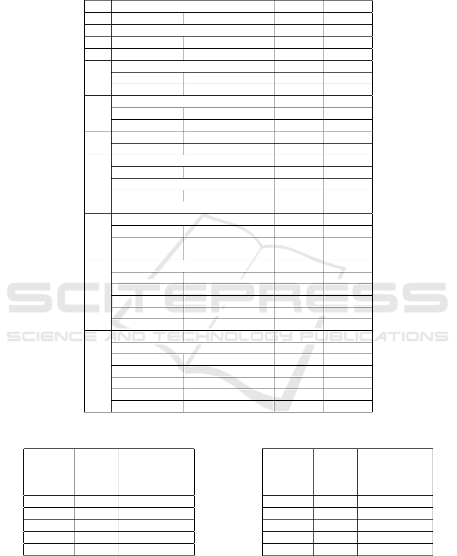
Table 9: Summary of Calculation Results The Economics of BM1 and BM2 wells.

No. Parameter Satuan Jumlah

1 Oil Production MMBBL 0.139

2 Time oil production Year 2

3 Price (Bbl) US$/Bbl 52

4 Gross Revenue MMUS$ 7.213

FTP MMUS$ 1.443

Contractor FTP MMUS$ 0.386

Government FTP MMUS$ 1.056

Investment MMUS$ 0.150

Tangible MMUS$ 0.000

Intangible MMUS$ 0.150

Operating cost Operation MMUS$ 2.774

Abandonment MMUS$ -

Cost Recovery MMUS$ 2.924

(% Gross Revenue) % 41%

Unrecovered Cost -

(% Gross Revenue) % 0%

9 Investment Credit (IC) 10% MMUS$ -

Equity to be Split MMUS$ 2.846

Contractor Equity MMUS$ 0.762

Government

Equity

MMUS$ 2.083

Contractor Take

Net Cash Flow MMUS$ 0.553

(% Gross Revenue) % 8%

IRR % ¿ MARR

NPV @15% MUS$ 451.07

POT Year ¡ 1

DPI Fraksi 4.00

Government Take

FTP + Equity MMUS$ 3.140

Tax MMUS$ 0.434

Net Cash Flow MMUS$ 3.736

(% Gross Revenue) % 52%

NPV @10% MUS$ 3,05

Table 10: Sensitivity analysis to oil prices

Sensitivity

(%)

Oil

price

(US$)

NPV at

Discount

factor 15%

(US$)

80 41 296.01

90 46 380.59

100 52 451.07

110 57 521.55

120 62 592.03

4 CONCLUSIONS

Optimization of installed pumps by changing SL and

SPM on BM1 wells from N = 6 and SL = 100 to

Table 11: Sensitivity analysis to operational costs.

Sensitivity

(%)

Oil

price

(US$)

NPV at

Discount

factor 15%

(US$)

80 16 504.57

90 18 477.82

100 20 451.07

110 22 424.32

120 24 397.97

N = 7 and SL 100 production rates increased from

144 BFPD to 199 BFPD with EV = 80% while in

well BM2 from N = 8 and SL = 100 to N = 10

Analysis of Economy in the Improvement of Oil Production using Hydraulic Pumping Unit in X Field

107

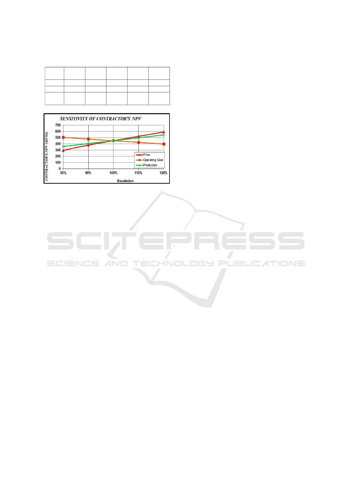
Table 12: Sensitivity analysis to production.

Years

80% 90% 100% 110% 120%

(Bbl/Y) (Bbl/Y) (Bbl/Y) (Bbl/Y) (Bbl/Y)

2017 58830 66190 73540 80890 88250

2018 52130 58650 65170 71680 78200

NPV

357.97 404.52 451.07 497.62 544.17

@15%

Figure 7: Sensitivity analysis.

and SL = 110 the production rate increased from

284 BFPD to 583 BFPD with EV = 90%. Based

on the results of production optimization for the next

2 years according to the time of HPU leasing, oil

production is 0.139 MMBBL, if it is assumed that

oil prices of US 52/BblareMMUS 7,213. Based

on the revenue sharing using the PSC system with

non-capital investments of MUS $ 0.150, the NPV

contractor MUS $ 451.07, IRR¿ MARR, POT <1

year and DPI 4.00 are obtained. From these results,

it can be seen for the next 2 years BM 1 and BM 2

wells are still economical to produce.

ACKNOWLEDGEMENTS

Thank you very much for supported by Universitas

Islam Riau and BOB PT. BSP Pertamina Hulu.

REFERENCES

Babbitt, J. A. and Vincent, K. (2012). Hydraulic Pumping

Units Proving Very Successful in Deliquifying Gas

Wells in East Texas. SPE Annual Technical

Conference and Exhibition.

Beard, D. (2013). Hydraulic pumping units proving

very successful in deliquifying gas wells in East

Texas. Society of Petroleum Engineers - North Africa

Technical Conference and Exhibition 2013, NATC

2013, 2.

Brown, K. E. (1984). The technology of artiﬁcial lift

methods, volume 4.

Chase, R. W. and Shaver, C. A. (2009). Optimal use of

vogel’s dimensionless ipr curve to predict current and

future inﬂow performance of oil wells. SPE Eastern

Regional Meeting, 295(5).

Cui, J., Xiao, W., Feng, H., Dong, W., Zhang, Y., and Wang,

Z. (2014). Long Stroke Pumping Unit Driven by

Low-Speed Permanent Magnet Synchronous Motor.

SPE Middle East Artiﬁcial Lift Conference and

Exhibition.

Hong, A., Bratvold, R. B., Lake, L. W., Maraggi,

R., and M., L. (2018). Integrating model

uncertainty in probabilistic decline curve analysis

for unconventional oil production forecasting.

SPE/AAPG/SEG Unconventional Resources

Technology Conference 2018, URTC 2018, (October

2018), 23–25.

Jennings, J. W. et al. (1989). The design of sucker rod

pump systems. In SPE Centennial Symposium at New

Mexico Tech. Society of Petroleum Engineers.

John, L. (1996). Decline Curve Analysis for Gas Wells.

Texas A&M University, College Station Texas.

Lubiantara, B. (2012). Ekonomi Migas Tinjauan Aspek

Komersial Kontrak Migas. Grasindo.

Ogunleye, A. O. (2012). Development of a Vogel type Inﬂow

Performance Relationship (IPR) for Horizontal wells.

SPE Annual Technical Conference and Exhibition.

Pickford, K. H. and Morris, B. J. (1989). Hydraulic rod

pumping units in offshore artiﬁcial lift applications.

SPE Production Engineering.

Wang, D. F., Cui, X. M., Gao, G. Y., Huang, Z. Z., and Hu,

B. Z. (1995). A New Long Stroke Pumping Unit with

High Speed. SPE Production Operations Symposium.

Wiggins, M. L., Russell, J. E., Jennings, J. W., et al.

(1996). Analytical development of vogel-type

inﬂow performance relationships. SPE Journal,

1(04):355–362.

Ye, Q., Wang, F., Wang, Y., Zhu, Y., Xu, J., Li, X.,

and Yang, G. (2017). Development and application

of pulley-free directly-connected hydraulic pumping

unit. Society of Petroleum Engineers - SPE/IATMI

Asia Paciﬁc Oil and Gas Conference and Exhibition

2017.

ICoSET 2019 - The Second International Conference on Science, Engineering and Technology

108