
Research of Intelligent Dynamic Dispathcing System of High Speed
and High Precision AGV
Liang Zhao
1, a
, Bin Cao
1
and Feng Lin
1
1
Department of Mechanical Engineering, Zhejiang University, Hangzhou, China
Keywords: Path planning, High speed high precision AGV, Astar algorithm, Scheduling system.
Abstract: In order to improve the working efficiency of high speed and high precision AGV, the method of path
planning in dispatching system is studied, and an improved Astar algorithm is proposed, which can reduce
the number of inflection points needed in path planning. The weight ratio of AGV going straight and turning
is raised. The improved algorithm is applied to AGV path planning, which improves the efficiency of the
algorithm. Experimental results show that the efficiency of this algorithm is higher than that of traditional
Astar algorithm in the application of specific enterprise projects.
1 INTRODUCTION
As a kind of automation equipment, AGV is
currently used in such process steps as material
transfer and parcel sorting in the workshop. During
the shopping festival, manual sorting cannot meet
the processing needs of a large number of orders,
and it is necessary to replace the manual with
automatic equipment [1]. Shi Jian Feng and Yang
Yong Sheng et al. (Shi Jianfeng, Yang Yongsheng,
2016) proposed an improved Dijkstra algorithm
which added parameters such as turning cost, energy
consumption cost, path patency and so on, reducing
the number of turns in path planning and improving
the effectiveness. Cao You Hui, Wang Liang Xi et
al. (Cao Youhui, Wang Liangxi, 2009) have made
the orientation of the target point dynamic, made the
combined force of gravitational repulsion is not
equal to zero, and avoided the defect that traditional
artificial potential field method is easy to fall into
the local minimum, and the good path planning of
AGV is realized. Wang Ding et al. (Wang Ding,
2008) used Astar algorithm to carry out the path
planning of AGV and modularized the scheduling
system, which reduced the cost of software
maintenance.
The research on scheduling strategy of AGV
mainly includes task assignment and path planning
(Lu Xinhua, Zhang Guilin, 2003; Huang Yuqing,
LIANG Liang, 2006; Huang Jiansheng, 2008). At
present, the research on path planning at home and
abroad mainly use algorithms such as Astar
algorithm, artificial potential field method, Dijkstra
algorithm (Ammar A, Bennaceur H, Chaari I, et al,
2016).
Most of the research focuses on the theoretical
innovation and the improvement of the algorithm
structure, whereas does not consider the actual AGV
projects. The project R&D, maintenance cost and the
R&D cycle are supposed to be considered for AGV
in the actual project research. Therefore, based on
the existing research of AGV, future research on
AGV are suggested to combine with specific
projects, to be tested in practical applications, and to
be examined regarding the efficiency as the ultimate
goal. In this paper, an AGV path planning method
based on the improved Astar algorithm is proposed.
Combined with specific projects, the turning cost of
AGV is added to the evaluation function, and the
artificial potential field method is used to effectively
reduce the number of turns, from which the
efficiency of AGV in actual (Yang Lianchang,
2012).
2 MODEL ESTABLISHMENT
2.1 Map Construction
Figure 1 shows the actual workshop map of a
project. According to the actual project task book,
the size of the material in the drawing is 1100*1100
354
Zhao, L., Cao, B. and Lin, F.
Research of Intelligent Dynamic Dispathcing System of High Speed and High Precision AGV.
DOI: 10.5220/0008850603540359
In Proceedings of 5th International Conference on Vehicle, Mechanical and Electrical Engineering (ICVMEE 2019), pages 354-359
ISBN: 978-989-758-412-1
Copyright
c
2020 by SCITEPRESS – Science and Technology Publications, Lda. All rights reserved
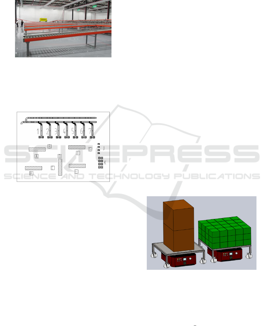
(mm), and the size of each sorting line is 5600*742
(mm). Each shipping port can accommodate no
more than 6 skips, the size of the delivery port area
is 3300*3300 (mm).
Figure 1. Layout of workshop.
The project is a typical medical material
distribution logistics system. The layout plan is
shown in Figure 2, and the map is rasterized to
facilitate the task assignment and the path to the
AGV. Planning.
Figure 2. CAD layout of workshop
In this figure, 1~7 are sorting lines. Each sorting
line corresponds to two picking points, A~H is the
delivery point. K is the empty storage area. J is the
charging pile and AGV waiting area. It makes full
use of idle time for charging and improve efficiency.
In this project, the work task of each AGV is to
transport the parcels of every sorting line from 1 to 7
to the designated position A~H. The task assignment
and path planning of the AGV are handled by the
on-site central dispatch system.
2.2 AGV Status Description
(1) As shown in the figure, the AGV comes with a
jacking device, therefore it can be transported from
the four directions of the skip to the bottom of the
skip. AGV’s movement will not be affected because
of its own universal wheels.
(2) Each time the AGV starts working in a point-
to-point state, the same car is not allowed to be sent
to different delivery points. The delivery port can
temporarily store the skip truck. If a temporary
storage area of a delivery port was full, no new task
would be sent to the delivery port.
(3) After the AGV delivery is completed, the
empty car leaves. Each delivery port sends an empty
vehicle recovery task request after the delivery is
completed. If it was less than two picking line
picking trucks, AGV would give priority to the
empty picking line to the picking line; otherwise, the
AGV would send the empty picking cart to the
staging area.
(4) Task assignment is divided into two ways. 1.
After the skip is full, the transport request is sent.
After the dispatch system acquires the mission
information, it assigns the corresponding AGV to
execute. 2. The caller manually calls to avoid the
cargo accumulation.
(5) If the number of empty pick-up trucks in a
sorting line was less than two, the dispatching
system would automatically deliver the empty-car
transport task.
(6) Set the charging post in the AGV waiting
area. If there was no task at a certain moment, the
AGV would automatically return to the waiting area
for charging. At any time during the waiting process,
only the voltage was not lower than the protection
voltage, and new tasks could be accepted.
(7) If the AGV voltage was lower than the
protection voltage, the charging task was
automatically executed after completing its own
task, and the AGV does not perform other tasks
during this process.
Figure 3. Schematic diagram of AGV transport skip.
2.3 AGV Mathematical Model
As shown in figure 4, the travel speed of the AGV
can be expressed as:
(1)
Research of Intelligent Dynamic Dispathcing System of High Speed and High Precision AGV
355
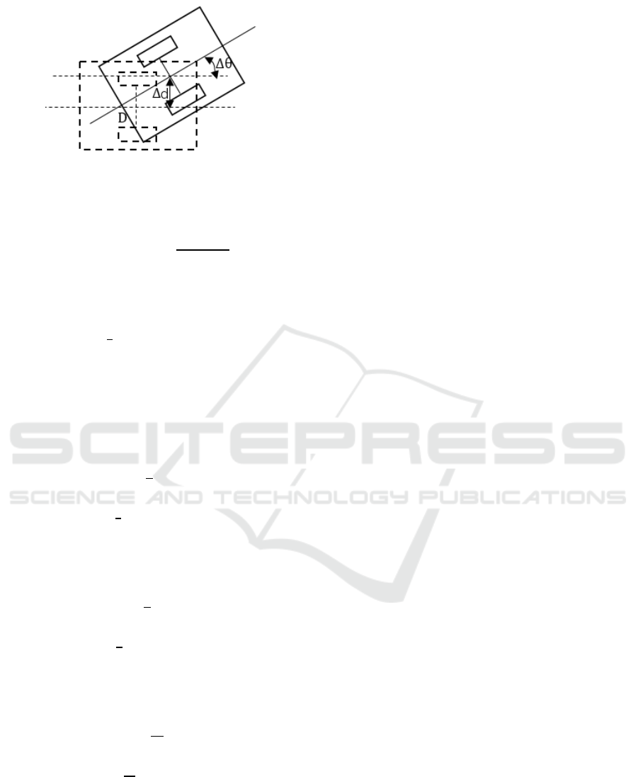
Figure 4. Model diagram of AGV.
The yaw angle ∆ can be expressed as:
∆ ∆
∙∆
(2)
The lateral offset distance ∆ is:
∆
∙∆∙∆
∙∆∙∆
(3)
Among them, the interval time between the two
gestures is ∆. The left drive wheel velocity is
,
The right drive wheel velocity is
, The centre
velocity is
, and the drive wheel pitch is .
Differentiate via time, get:
∆
(4)
∆
∆
(5)
To integrate by t can get the equation of motion
of the AGV during driving:
(6)
∆ ∙
(7)
Finally, the Laplace transform is performed on
the time:
(8)
(9)
2.4 System Mathematical Model
Suppose that m tasks are performed by n AGVs in a
certain period of time, the time taken for each AGV
to complete its task is
1…. In order to
make the task assignment more uniform and the
system more efficient,
must be the
smallest.
The number of AGVs is N, the total number of
tasks is M (s). The number of sorting lines is c
(strips). The number of delivery ports is b (several).
Each delivery port temporary storage area can be
stocked by e (s). The AGV rated load is W (kg). The
actual load of task i is w_i(kg). The time of AGV
from the sorting line to the delivery port in task i is
t_i(s).
At the same time, the decision variable is defined
as
: When the AGV k executing the task i after
the task j, the value is 1, otherwise it is 0;
: When
the task i is executed by the AGV k, the value is 1,
otherwise it is 0. According to the project
description, a mathematical model of the multi-AGV
scheduling system is established as:
∈
1,2,⋯
(10)
..
,∈
1,2,⋯
(11)
∑
, 0
1, 1,2,,,
(12)
∑
,∈
0,1,,,
,∈
0,1,,,
(13)
The constraint conditions combine the mission
status and travel of the AGV: 1. The AGV load must
not exceed the rated load; 2. A task can only be
executed by one AGV; 3. The AGV performs only
one task before performing the current task.
3 IMPROVED ASTAR
ALGORITHM
3.1 Artificial Potential Field Method
The artificial potential field method can predict
obstacles in advance. It is assumed that the obstacle
generates a repulsive force to the moving object, and
the target point generates gravity to the moving
object in the artificial potential field method, thereby
it will avoid the situation that the AGV hits the
obstacle and then turns to effectively reduce the
number of inflection point.
ICVMEE 2019 - 5th International Conference on Vehicle, Mechanical and Electrical Engineering
356
In order to combine the Astar algorithm, this
paper makes the following changes:
(1) Only the repulsive field is retained, and the
heuristic function h(n) in Astar replaces the role of
the gravitational field.
(2) By classifying the repulsion and the
extended, only the direction in which the nodes are
extended is opposite to the repulsion is reserved.
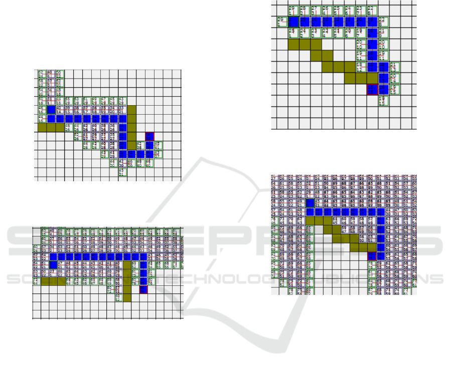
Table 1. Comparison between traditional algorithm and
improved with the artificial potential field method.
Case 1
Walking path length: 18 nodes
Turning times: 4
Case 2
Walking path length: 16 nodes
Turning times: 2
Case 1 is the path planning of the traditional
Astar algorithm, and case 2 is the path obtained by
adding the artificial potential field method. It can be
seen that the traditional Astar may increase the
number of inflection points toward the obstacle
movement, and if the obstacle can be bypassed at the
start, the inflection points’ number is reduced.
3.2 The Turn Cost
Add the turn cost in the actual cost, assuming that
the cost of rotating in situ at a node is α times to the
straight walk, so there are:
α
1α
(14)
The path obtained by improved Astar algorithm
with the turning cost is as shown in the table 2:
Table 2. Comparison between traditional algorithm and
improved with the turn cost.
Case 1
Walking path length: 15 nodes
Turning times: 4
Case 2
Walking path length: 15 nodes
Turning times: 3
The traditional Astar algorithm has a large
number of inflection points. After adding the turning
cost and the number of inflection points to the
evaluation function, it will effectively reduce the
number of turns and improve the efficiency.
4
THEORETICAL
VERIFICATION
Intuitively using the presentation software to
demonstrate the performance of improved
algorithms, analyze the number of inflection points,
path lengths, and analyze the final path of the
traditional Astar algorithm and its improved
algorithm and compare the validity and correctness
of the final path results.
The six experimental maps followed are used for
verification:
Research of Intelligent Dynamic Dispathcing System of High Speed and High Precision AGV
357
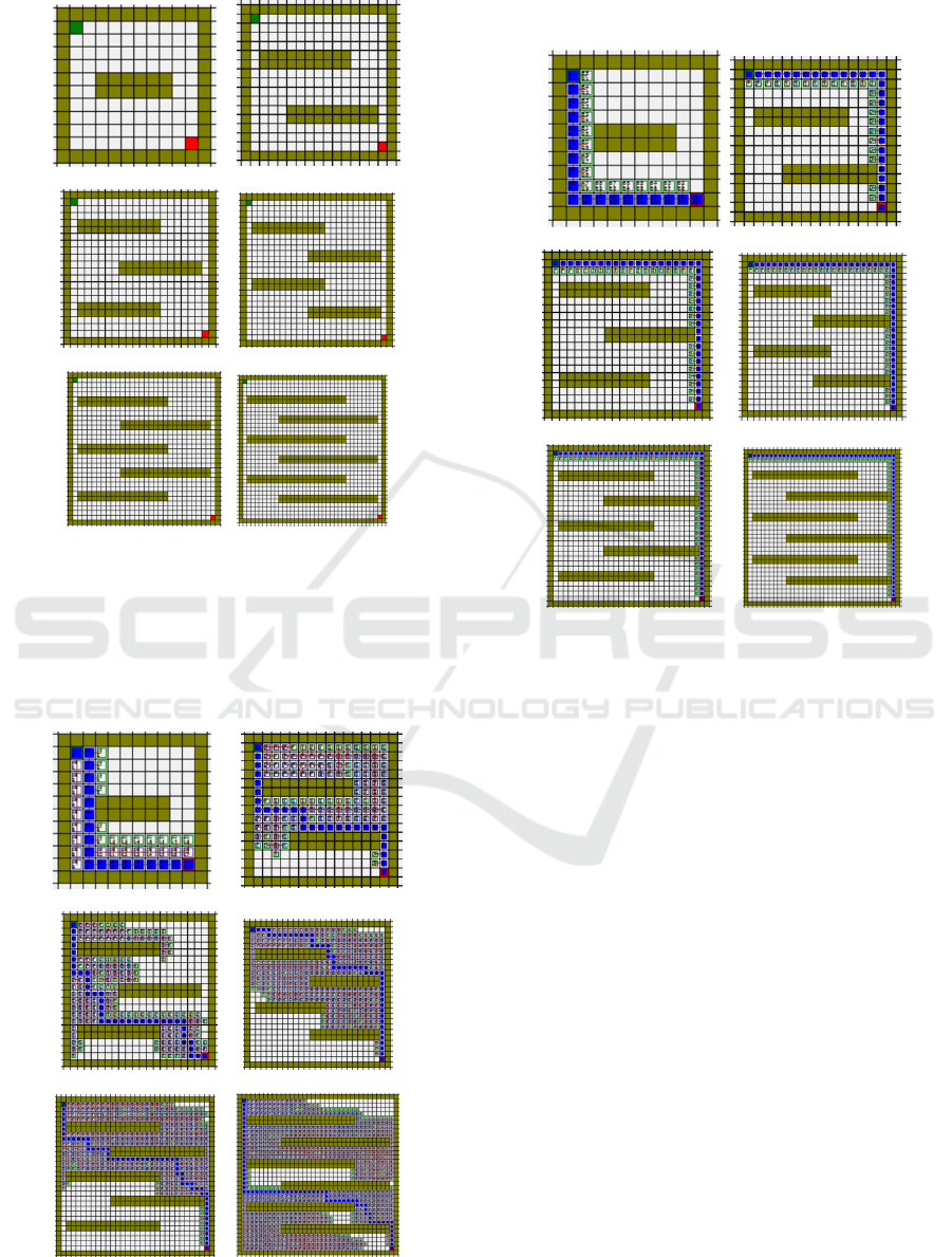
Table 3. Experimental maps.
10*10 15*15
20*20 25*25
30*30 35*35
After testing the feasibility of the improved
algorithm with different number of nodes, the path
plan obtained by the traditional Astar algorithm is
shown in the table 4:
Table 4. The path obtained by traditional algorithm.
10*10 15*15
20*20 25*25
30*30 35*35
The improved algorithm gets the path as shown:
Table 5. The path obtained by improved algorithm.
10*10 15*15
20*20 25*25
30*30 35*35
By comparing the path length and the number of
inflection points, the analysis results are shown in
the table 6:
5
CONCLUSIONS
(1) The traditional Astar algorithm is based on the
grid map, with the evaluation function as the core,
and the shortest path is foreseen. However, it cannot
predict the location of obstacles in advance. It has
low predictability, and does not recognize the cost of
turning in actual projects.
(2) Adding the artificial potential field method to
predict the position of obstacles can greatly improve
the predictability of the algorithm, reduce the
number of inflection points in the path, and improve
efficiency in the actual project.
(3) Adding the turning cost is more suitable for
the path planning in the actual project, the operation
and path planning simulation of the mobile robot.
The number of inflection points in the path can be
stably reduced and the work efficiency can be
greatly improved.
ICVMEE 2019 - 5th International Conference on Vehicle, Mechanical and Electrical Engineering
358

Table 6. Path analysis of traditional algorithm and
improved algorithm.
Map Project
Traditional
Astar
Improved
Astar
Map 1
(10*10)
Turning
times
2 1
Walking
path
length
18 18
Map 2
(15*15)
Turning
times
4 1
Walking
path
length
28 28
Map 3
(20*20)
Turning
times
9 1
Walking
path
length
38 38
Map 4
(25*25)
Turning
times
11 1
Walking
path
length
48 48
Map 5
(30*30)
Turning
times
14 1
Walking
path
length
58 58
Map 6
(35*35)
Turning
times
10 1
Walking
path
length
68 68
REFERENCES
Ammar A, Bennaceur H, Chaari I, et al. Relaxed Dijkstra
and A* with linear complexity for robot path planning
problems in large-scale grid environments [J]. Soft
Computing, 2016, 20(10):4149-4171.
Cao Youhui, Wang Liangxi. Study on local path planning
of AGV based on virtual target [J]. Computer
simulation, 2009, 26(1):162-165.
Core capabilities, functional positioning and development
strategy of China's manufacturing industry -- and
comments on "made in China 2025" [J]. China
industrial economy, 2015(6):5-17.
Huang Jiansheng. Path planning of mobile robot [D].
School of information science and engineering,
zhejiang university, 2008.
Huang Yuqing, LIANG Liang. Path planning algorithm in
robot navigation system [J]. Journal of microcomputer
information, 2006, 22(20):259-261.
Lu Xinhua, Zhang Guilin. Research on indoor service
robot navigation method [J]. Robot, 2003, 25(1):80-
87.
Shi Jianfeng, Yang Yongsheng. AGV path planning based
on improved Dijkstra algorithm [J]. Science and
technology vision, 2016(20):111-112.
Wang Ding. Research on AGV scheduling system and
path planning [D]. Shandong University, 2018.
Yang Lianchang. Interpretation of the development
roadmap of intelligent manufacturing equipment
during the 12th five-year plan period [J]. China
electrical equipment industry association, 2012: 17-19.
Research of Intelligent Dynamic Dispathcing System of High Speed and High Precision AGV
359
