Taming Complexity with Self-managed Systems

Daniel A. Menasc

Department of Computer Science, George Mason University, Fairfax, VA, U.S.A.

Keywords:

Autonomic computing, self-managed Systems, Utility Functions.

Abstract:

Modern computer information systems are highly complex, networked, have numerous conﬁguration knobs,

and operate in environments that are highly dynamic and evolving. Therefore, one cannot expect that conﬁg-

urations established at design-time will meet QoS and other non-functional goals at run-time. For that reason,

the design of complex systems needs to incorporate controllers for adapting the system at run time. This pa-

per describe the four properties of self-managed systems: self-conﬁguring, self-optimizing, self-healing, and

self-protecting. It also describes through concrete examples how these properties are enforced by controllers

I designed for a variety of domains including cloud computing, fog/cloud computing, Internet datacenters,

distributed software systems, and secure database systems.

1 INTRODUCTION

Modern computer systems are networked, are com-

posed of a very large number of interconnected

servers, have many software layers that may include

services developed by many different vendors, are

composed of hundreds of thousands of lines of code,

and are user-facing. Additionally, these systems have

stringent Quality of Service (QoS) requirements in

terms of response time, throughput, availability, en-

ergy consumption, and security. These systems have

a very large number of conﬁguration settings that sig-

niﬁcantly impact their QoS behavior.

This complexity is compounded by the fact that

the workload intensity of these complex systems

varies in rapid and hard-to-predict ways.

For these reasons, it is virtually impossible for

human beings to change the conﬁguration settings

of a complex system in near real-time in order to

steer the system to an optimal operating point that

meets user-established QoS goals. Recognizing this,

IBM introduced the concept of autonomic comput-

ing, as a sub-discipline of computer science that

deals with systems that are self-conﬁguring, self-

optimizing, self-healing, and self-protecting (Kephart

and Chess, 2003). Autonomic computing systems are

also referred to as self-managed systems.

The rest of this paper is organized as follows. Sec-

tion 2 describes the basics of self-managed systems.

Section 3 discusses how an autonomic controller can

https://orcid.org/0000-0002-4085-6212

be used to provide elasticity to cloud providers al-

lowing them to cope with workload surges by dy-

namically varying the number of servers offered to

users. Section 4 provides an example of how an auto-

nomic controller can deal with tradeoffs between se-

curity and response time by dynamically varying the

security policies of an Intrusion Detection and Pre-

vention Systems (IDPS). The next section discusses

how an autonomic controller can dynamically control

the voltage and frequency of a CPU in order to meet

performance requirements with the least possible en-

ergy consumption. Section 6 provides a list of other

examples of self-managed systems. Finally, Section 7

provides some concluding remarks.

2 BASICS OF SELF-MANAGED

SYSTEMS

This section discusses the basics of self-managed

systems aka autonomic computing systems, a term

coined by IBM (Kephart and Chess, 2003) more than

a decade ago. The term autonomic computing was

inspired by the central autonomic nervous system,

which unconsciously regulates bodily functions such

as the heart and respiratory rate, digestion, and others.

Figure 1 illustrates the basic components of a self-

managed system. The system to be controlled is sub-

ject to a workload that consists of the sets of all in-

puts to the system (e.g., requests, transactions, web

requests, and service requests). The output metrics

MenascÃl’, D.

Taming Complexity with Self-managed Systems.

DOI: 10.5220/0008346100050013

In Proceedings of the 21st International Conference on Enterprise Information Systems (ICEIS 2019), pages 5-13

ISBN: 978-989-758-372-8

!"#$%&'$(')%''

*(+$,(--%.'

/(+$,(--%,'

!"#$%"&'(

")*+)*(,-*#./0(

1.213%-4-%(2"&%0(

%"!3%-4-%((

/"5*#"%0(

Figure 1: Basic components of a self-managed system.

of the system are associated with the QoS delivered

by the system when processing the inputs. Exam-

ples of output metrics are: (a) 95% of web requests

have a response time less than or equal to 0.8 sec; (b)

the average search engine throughput is at least 4,600

queries/sec; (c) the availability of the e-mail portal is

greater than or equal to 99.978%; and (d) the percent-

age of phishing e-mails ﬁltered by the e-mail portal is

greater than or equal to 90%.

Figure 1 also depicts a controller that monitors

the system input, i.e., the workload, its output met-

rics, and compares the measured output metrics with

high-level goals established by the system stakehold-

ers. The controller reacts to deviations from the de-

sired QoS levels established by the stakeholders by

automatically deriving a plan to change the system’s

conﬁguration by changing low-level controls in a way

that improves the system’s QoS and makes it compli-

ant, if the system resources permit, with the high-level

goals.

Self-managed systems work along the following

dimensions: (a) Self-conﬁguring: The system auto-

matically decides how to best conﬁgure itself when

new components or services become available or

when existing ones are decommissioned. (b) Self-

optimizing: The system attempts to optimize the value

of its QoS metrics (e.g., minimizing response time,

maximizing throughput and availability). (c) Self-

healing: The system has to automatically recover

from failures. This requires that the root causes of

failures be determined and that recovery plans be de-

vised to restore the system to an adequate operational

state. In addition, the system has to predict the occur-

rence of failures and prevent their manifestation. (d)

Self-protecting: The system has to be able to detect

and prevent security attacks, even zero-day attacks,

i.e., attacks that target publicly known but still un-

patched vulnerabilities.

Optimizing a system for the four dimensions

above may be challenging because there are tradeoffs

among them. For example, it may be necessary to

add several cryptographic-based defenses to improve

a system’s security. However, these defenses have a

computational cost and increase the response time and

decrease the throughput (Menasc

e, 2003). As another

example, one may increase the reliability of a sys-

tem, and therefore improve its self-healing capabili-

ties, by using redundant services with diverse imple-

mentations. However, this approach tends to increase

response time.

In addition, there usually are constraints in terms

of cost and/or energy consumption associated with

this optimization problem, which has to be solved

in near real-time to cope with the rapid variations of

the workload. This problem is a multi-objective opti-

mization problem (Miettinen, 1999). In order to deal

with the tradeoffs, it is common to use utility func-

tions for each metric of interest and then combine

them into a global utility function to be optimized.

A utility function indicates how useful a system

is with respect to a given metric. Utility functions

are normalized (in our case in the [0,1] range) with 1

indicating the highest level of usefulness and 0 the

lowest. For example, if the metric is response time,

the utility function of the response time decreases as

the response time increases, and approaches 1 as the

ICEIS 2019 - 21st International Conference on Enterprise Information Systems

response time decreases. As another example, a util-

ity function of availability increases as the availability

increases.

We assume here that all utility functions are con-

sistent, i.e., they increase or decrease in the right di-

rection according to the metric. So, a utility function

that increases as the response increases is not consis-

tent. Figure 2 shows examples of utility functions.

The lefthand side of the ﬁgure shows three different

functions with different shape factor (α) but with the

same service level goal (β = 65.0), which is the in-

ﬂection point of the curve. The righthand side of

Fig. 2 shows three different availability utility func-

tions. The inﬂection point is the same for all of them,

i.e., 0.99.

The controller of Fig. 1 typically awakes at regu-

lar time intervals, called controller intervals and de-

noted as ∆. Then, the controller (a) veriﬁes all the

monitoring data collected during the past controller

interval(s), (b) analyzes how the measured output

metrics compare with the high-level goals, (c) gen-

erates, if necessary, a plan to change the conﬁgu-

ration controls to bring the system in line with the

high-level goals, and (d) executes the plan by send-

ing commands to the system. The plan is generated

based on knowledge of models of the system behav-

ior, which will guide the generation of new conﬁgu-

ration parameters as explained in what follows. The

paradigm described above is called MAPE-K, which

stands for Monitor, Analyze, Plan, and Execute based

on Knowledge (Kephart and Chess, 2003).

We formalize now the operation of an autonomic

controller (just controller heretofore). To that end we

deﬁne the following notation.

• K: number of conﬁguration knobs (low level con-

trols in Fig. 1) the controller is able to change.

•

C(t) = (C

,··· ,C

): vector of values of the K

conﬁguration knobs at time t.

• C : set of all possible vectors

C(t).

• W (t): workload intensity at time t. This is usu-

ally the workload intensity in the last controller

interval but could also be a predicted workload for

the next controller interval.

• S(t) = (

C(t),W (t)): system state at time t, which

consists of the system conﬁguration and the work-

load at time t.

• m: number of ouput metrics monitored by the con-

troller.

• D

: domain of metric i.

• x

(t) ∈ D

: value of metric i (i = 1, ··· , m) at

time t.

• g

(S(t)): function used to compute (i.e., esti-

mate) the value of metric i at time t. So, x

(t) =

(S(t)) = g

((

C(t),W (t)). The function g

() rep-

resents a model of the system being controlled. In

virtually all cases of interest, the functions g

() are

non-linear.

• U

) ∈ [0, 1]: utility function for metric i. This is

a function of the values of metric i.

• U

,··· , x

) = f (U

),··· ,U

)): global

utility function, which is a function of all individ-

ual utility functions.

The functions g

(),··· , g

() are typically analytic

models used to estimate the values of each of the m

metrics as a function of the current or future system

state S(t). The functions U

(), i = 1,··· , m and U

()

are the high-level goals and are determined by the

stakeholders.

At any time instant t at which the controller wakes

up, it selects values for the conﬁguration parameters

that will be in place from time t to time t + ∆, when

the controller will wake up again and possibly make

another selection of parameters.

Because the global utility function is a function

of the values of the metrics (i.e., U

,··· , x

))

and because each value x

is a function g

(S(t)) =

((

C(t),W (t)) of the system parameters, the con-

troller needs to ﬁnd a conﬁguration vector

∗

(t) that

maximizes the global utility function. More precisely,

∗

(t) = argmax

∀

C(t)∈C

{ f (U

((

C(t),W (t))),

··· ,U

((

C(t),W (t))))}

In many cases we may want to add constraints

such as a cost constraint: Cost(

C(t)) ≤ CostMax

It should be noted that complex computer systems

have a large number of conﬁguration knobs and the

number of possible values of each is usually large.

Therefore, we have a combinatorial explosion in the

cardinality of C .

Additionally, the solution of the optimization

problem stated above has to be obtained in near-

real time. For this reason, we often resort to the

use of combinatorial search techniques such as hill-

climbing, beam-search, simulated annealing, and evo-

lutionary computation to ﬁnd a near-optimal solution

in near real-time (Ewing and Menasc

e, 2014).

3 TAMING WORKLOAD SURGES

Most user-facing systems such as Web sites, social

network sites, and cloud providers suffer from the

phenomenon of workload surges (aka ﬂash crowds),

Taming Complexity with Self-managed Systems

0.2

0.4

0.6

0.8

0 20 40 60 80 100 120

Utility

Execution Time

α = 0.05, β = 65.0

α = 0.15, β = 65.0

α = 0.50, β = 65.0

0.2

0.4

0.6

0.8

0.97 0.975 0.98 0.985 0.99 0.995 1

Utility

Availability

α = -1500, β = 0.99

α = -500, β = 0.99

α = -200, β = 0.99

Figure 2: Left side: examples of utility functions for execution time. Right side: examples of utility functions for availability.

All examples are sigmoid functions.

i.e., periods of relatively short duration during which

the arrival rate (measured in arriving requests per sec-

ond) exceeds the system’s capacity (measured in the

maximum number of requests per second that can be

processed). The ratio between the average arrival rate

of requests and the system’s capacity is called trafﬁc

intensity and is typically denoted by ρ in the queuing

literature. A queuing system is in steady-state when

ρ < 1.

The top of Fig. 3 illustrates an example of a work-

load intensity surge from traces publicly made avail-

able by Google. As the ﬁgure illustrates, the surge

occurs in the interval between 600 sec and 1,500 sec,

during which time the workload intensity increased

by a 4.5 factor: from an average of 0.2 requests/sec

to 0.9 requests/sec. The peak of the surge occurred at

time equal to 1,200 sec. The middle curve of Fig. 3

shows that the response time increased from its pre-

surge value of 10 sec to a peak value of 375 sec, i.e.,

a 37.5-fold increase. Additionally, the peak response

time caused by the surge occurred at 1,600 sec, i.e.,

300 sec after the peak of the surge occurred.

The bottom part of Fig. 3 shows various curves

obtained by using an elasticity controller that uses an

analytic model used to predict the response time of a

multi-server queue under surge conditions (i.e., when

ρ > 1) (Tadakamalla and Menasc

e, 2018). This model

establishes a relashionship between the maximum de-

sirable response time, the trafﬁc intensity, and param-

eters that determine the geometry of the surge (the red

curve in the bottom ﬁgure is a trapezoidal approxima-

tion of the surge in the top ﬁgure). The cyan curve

is a predicted response time curve based on the trape-

zoidal approximation and is obtained from the ana-

lytic model.

The autonomic controller monitors the trafﬁc in-

tensity ρ at regular intervals and detects when it ex-

ceeds 1. At this point it uses the model to compute

the minimum number of servers needed to bring down

the response time. Every time the controller wakes up

and notices that ρ > 1 it adjusts the number of needed

servers. The green step curve in the bottom of Fig. 3

shows that the system capacity increased twice during

the surge and that the response time (see blue curve at

the bottom of Fig. 3) reached at most 50 sec instead

of 375 sec without the controller.

4 AUTONOMIC INTRUSION

DETECTION PREVENTION

SYSTEMS

As indicated in Section 2, the properties of self-

managed systems include self-optimizing and self-

protecting. In this section, we present an example of

a work (Alomari and Menasc

e, 2013) that discusses

the design, implementation, and use of an autonomic

controller to dynamically adjust the security policies

of an Intrusion Detection Prevention System (IDPS).

There are two types of IDPSs: data-centric and

syntax-centric. The former type inspects the data

coming from a backend database to a client and de-

termines if the security policies of the IDPS allow the

requesting user to receive the data. The latter, inspects

the syntax of SQL requests and determines if the se-

curity policies of the IDPS allow the requesting user

to submit that request. Because no IDPS is able to

cover all types of possible attacks, many systems use

several data-centric and several syntax-centric IDPSs.

So, an incoming request will have to be processed

by several syntax-centric IDPSs of different types and

an outgoing response will have to be handled by sev-

eral different data-centric IDPSs. While this process

increases the security of a system, it may severely de-

grade its performance.

For example, when a system is under a high work-

load, it might be acceptable to modify the security

ICEIS 2019 - 21st International Conference on Enterprise Information Systems

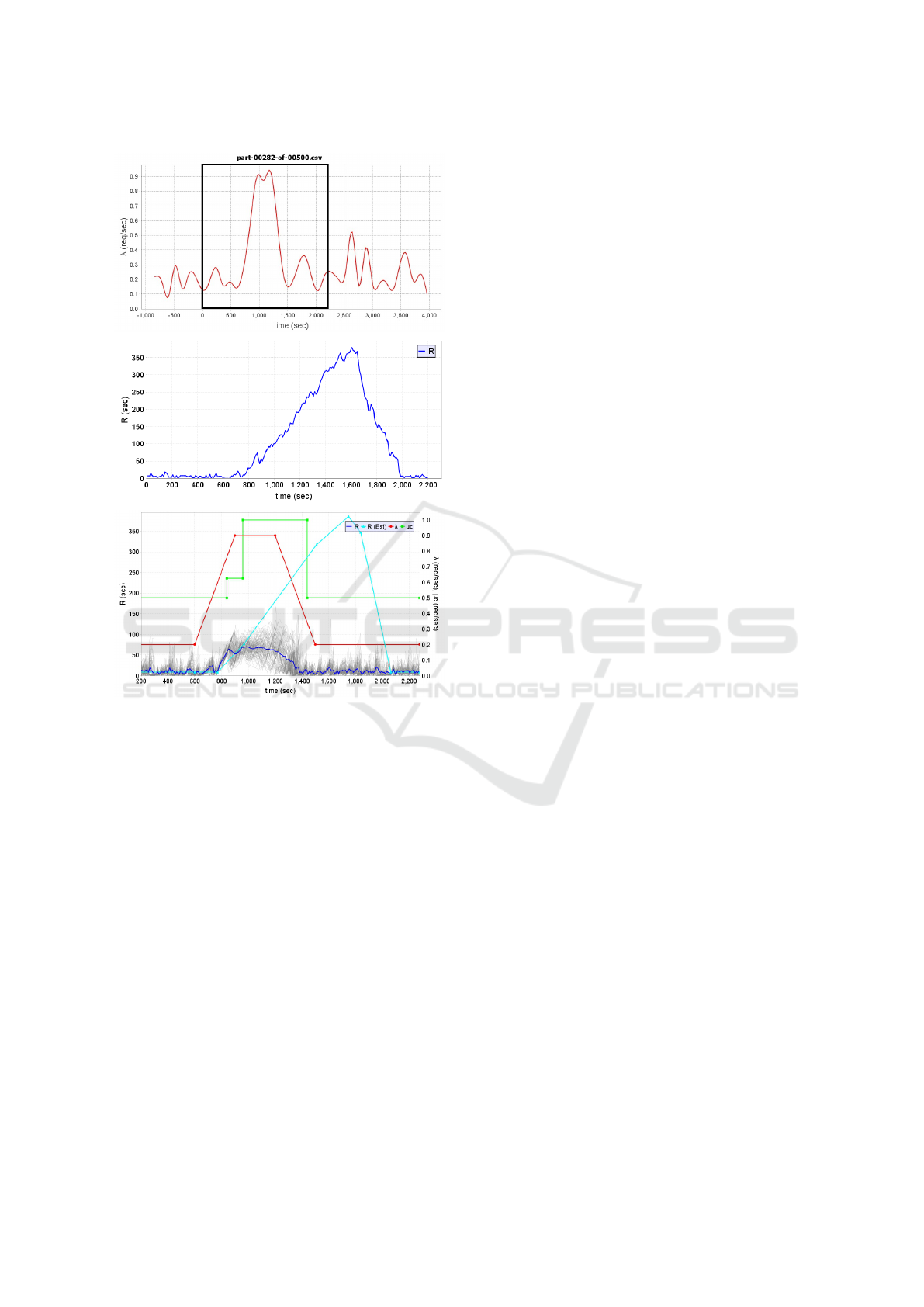
Figure 3: (a) Top – Example of a trapezoidal workload

surge from Google’s cluster-usage trace ﬁle, part-00282-of-

00500.csv; workload surge period: 600-1,500 sec; average

arrival rate before and after surge: 0.2 requests/sec; maxi-

mum arrival rate during surge: 0.9 requests/sec; (b) Mid-

dle – System’s response time for the duration correspond-

ing to the black highlighted box from the top ﬁgure; (c)

Bottom – Red curve: approximated trapezoidal workload;

Green curve: total server capacity; Cyan curve: Estimated

response time curve based on the red curve; Blue curve:

Response time with the controller averaged over 100 inde-

pendent runs using the Google trace workload in part (a)

above. See (Tadakamalla and Menasc

e, 2018).

policies to relax some of the security requirements

temporarily to meet increasing demands. Addition-

ally, since in most situations, different system stake-

holders view priorities differently, the relaxation in

security requirements should ideally be based on pre-

deﬁned stakeholder preferences and risks.

We designed an autonomic controller that dynam-

ically changes the system security policies in a way

that maximizes a utility function that is the combina-

tion of two utility functions: one for performance and

another for security (Alomari and Menasc

e, 2013).

The former is a function of the predicted response

time and the latter is a function of the detection rate

and false positive rate. Users are classiﬁed into roles

and security policies are associated with the different

roles. A security policy for a role r is deﬁned as a vec-

tor

= (ε

r,1

,··· , ε

r,M

) where ε

r,i

= 0 if IDPS i is not

used for requests of role r and equal to 1 otherwise.

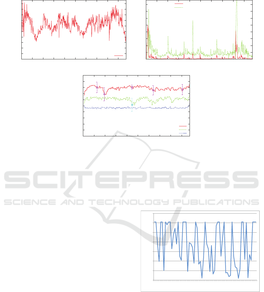
Figure 4 illustrates the results of experiments con-

ducted with the controller in a TPC-W e-commerce

site. The x-axis for all graphs is time measured in con-

troller intervals (i.e., the time during which the con-

troller sleeps).

The graph in Fig. 4 (a) illustrates the variation

of the workload intensity measured in number of re-

quests received by the system over time. As it can be

seen, the workload is very bursty and varies widely

(between 50 req/sec and 140 req/sec). The high work-

load peaks cause response time spikes that violate the

Service Level Agreements (SLA) of 1 second for ac-

cess to the home page and 3 seconds for search re-

quests as illustrated in Fig. 4 (b). Figure 4 (c) shows

three global utility curves. The top curve is obtained

when the controller is enabled and shows that the util-

ity is kept at around 0.8 despite the variations in the

workload. The middle curve is obtained when the

controller is disabled and the security policy is pre-

conﬁgured and does not change dynamically; in this

case the global utility is about 0.6. Finally, the bottom

curve is obtained when a full security policy (i.e., one

in which all IDPSs are enabled for all roles) is used.

In this case, a very low global utility of around 0.48 is

observed.

Thus, as Fig. 4 shows, the autonomic controller

is able to maintain the global utility at a level 67%

higher than when the all IDPSs are enabled by re-

ducing the security policies when the workload goes

through periods of high intensity.

5 AUTONOMIC

ENERGY-PERFORMANCE

CONTROL

Power consumption at modern data centers is now

a signiﬁcant component of the total cost of owner-

ship. Exact numbers are difﬁcult to obtain because

companies such as Google, Microsoft, and Amazon

do not reveal exactly how much energy their data

centers consume. However, some estimates reveal

that Google uses enough energy to continously power

200,000 homes (Menasc

e, 2015).

Most modern CPUs provide Dynamic Voltage and

Frequency Scaling (DVFS), which allows the pro-

Taming Complexity with Self-managed Systems























         

























         





!"

#!"























         









 !

"!

Figure 4: Experiment results (see (Alomari and Menasc

e, 2013)): (a) (top-left) Workload variation, (b) (top right) Response

time for Home and Search page requests without the controller, (c) (bottom) Three global utility values: with the controller,

for a ﬁxed pre-conﬁgured policy, and for a full security policy.

cessor to operate at different levels of voltage and

clock frequency values. Because a processor’s dy-

namic power is proportional to the product of the

square of its voltage by its clock rate, it is possi-

ble to control the power consumed by a processor by

dynamically varying the clock frequency. However,

lower clock frequencies imply in worse performance

and higher clock rates improve the processor’s perfor-

mance. Therefore, it would be ideal to dynamically

vary a processor’s clock rate so that as the workload

intensity increases, the clock rate is increased to meet

response time SLAs. And, as the workload intensity

decreases the clock frequency should be decreased to

the lowest value that would maintain the desired SLA

so as to conserve energy.

Many microprocessors allow for states in which a

different voltage-frequency pair is allowed. For ex-

ample, the Intel Pentium M processor supports the

following six voltage-frequency pairs: (1.484 V, 1.6

GHz), (1.420 V, 1.4 GHz), (1.276 V, 1.2 GHz), (1.164

V, 1.0 GHz), (1.036 V, 800 MHz), and (0.956 V, 600

MHz) (Intel, 2004). As indicated above, micropro-

cessors with DVFS offer a discrete set of voltage-

frequency pairs.

We designed and experimented with an autonomic

DVFS controller that dynamically adjusts the voltage-

frequency pair of the CPU to the lowest value that

meets a user-deﬁned response time SLA (Menasc

2015).

Figure 5 illustrates an example of the variation of

the average arrival rate (λ) over time. As it can be

seen, the workload intensity varies widely between

0.01 tps and 0.61 tps.

!"!#

!"$#

!"%#

!"&#

!"'#

!"(#

!")#

!"*#

$# &# (# *# +# $$#$&#$(#$*#$+#%$#%&#%(#%*#%+#&$#&&#&(#&*#&+#'$#'&#'(#'*#'+#($#(&#((#(*#(+#)$#)&#

)(#

!"#$%&#'!$$("%)'$%*#'+*,-.'

/(0#'12*#$"%)-'

Figure 5: Average Transaction Arrival Rate (in tps) vs.

Time Intervals.

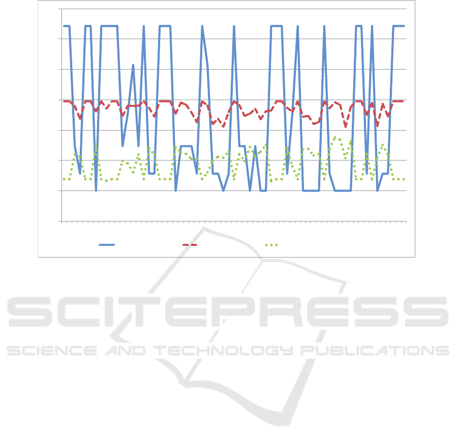
The DVFS autonomic controller is able to react to

these variations as shown in Fig. 6 that shows three

different curves. The x-axis follows the same time in-

tervals as in Fig. 5 but the scale on that axis is labelled

with the values of λ over the interval. The solid curve

shows the variation of the relative power consumption

that results from the variation of the voltage and CPU

clock frequencies. We deﬁne the relative power con-

ICEIS 2019 - 21st International Conference on Enterprise Information Systems

sumption as the ratio between the power consumed by

the processor for a given pair of voltage and frequency

values and the lowest power consumed by the proces-

sor, which happens when the lowest voltage and fre-

quencies are used.

As can be seen, the shape of the relative power

curve follows closely the variation of the workload

intensity. Higher workload intensities require higher

CPU clock frequencies and voltage levels and there-

fore higher relative power consumption. The dashed

curve of Fig. 6 shows the variation of the average re-

sponse time over time. The ﬁrst observation is that the

average response time never exceeds its SLA of 4 sec.

The response time, given that the I/O service demand

is ﬁxed throughout the experiment, is a function of the

arrival rate λ and the CPU clock frequency during the

time interval. This curve and the dotted line (i.e., the

CPU residence time) in the same ﬁgure clearly show

how the autonomic DVFS controller does its job.

6 OTHER EXAMPLES OF

SELF-MANAGED SYSTEMS

Self-managed systems have been used in a wide vari-

ety of systems in addition to the examples discussed

above. In (Tadakamalla and Menasc

e, 2019), the

authors discuss an autonomic controller that dynam-

ically determines the portion of a transaction that

should be processed at a fog server vs. at a cloud

server. The controller deals with tradeoffs between lo-

cal processing (less wide area network time but higher

local congestion) and remote processing (more wide

area network trafﬁc but use of more powerful servers

and therefore less remote congestion).

The authors in (Bajunaid and Menasc

e, 2018)

show how one can dynamically control the check-

pointing frequency of processes in a distributed sys-

tem so as to balance execution time and availability

tradeoffs.

The work in (Connell et al., 2018) presents ana-

lytic models of Moving Target Defense (MTD) sys-

tems with reconﬁguration limits. MTDs are security

mechanisms that periodically reconﬁgure a system’s

resources to reduce the time an attacker has to learn

about a system’s characteristics. When the reconﬁgu-

ration rate is high, the system security is improved at

the expense of reduced performance and lower avail-

ability. To control availability and performance, one

can vary the maximum number of resources that can

be in the process of being reconﬁgured simultane-

ously. The authors of (Connell et al., 2018) devel-

oped a controller that dynamically varies the max-

imum number of resources being reconﬁgured and

the reconﬁguration rate in order to maximize a util-

ity function of performance, availability, and security.

The Distributed Adaptation and REcovery

(DARE) framework designed at Mason (Albassam

et al., 2017) uses a distributed MAPE-K loop to

dynamically adapt large decentralized software

systems in the presence of failures. The Self-

Architecting Service-Oriented Software SYstem

(SASSY) project (Menasc

e et al., 2011), also de-

veloped at Mason, allows for the architecture of

an SOA system to be automatically derived from a

visual-activity based speciﬁcation of the application.

The resulting architecture maximizes a user-speciﬁed

utility function of execution time, availabiliy, and

security. Additionally, run-time re-architecting

takes place automatically when services fail or the

performance of existing services degrades.

In (Menasc

e et al., 2015) the authors describe

how autonomic computing can be used to dynami-

cally control the throughput and energy consumption

of smart manufacturing processes.

The authors in (Aldhalaan and Menasc

e, 2014),

discuss the design and evaluation of an autonomic

controller that dynamically allocates and re-allocates

communicating virtual machines (VM) in a hierarchi-

cal cloud datacenter. Communication latency varies

if VMs are colocated in the same server, same rack,

same cluster, or same datacenter. The controller em-

ploys user-speciﬁed information about communica-

tion strength among requested VMs in order to de-

termine a near-optimal allocation.

The authors in (Ewing and Menasc

e, 2009) pre-

sented the detailed design of an autonomic load bal-

ancer (LB) for multi-tiered Web sites. They assumed

that customers can be categorized into distinct classes

(gold, silver, and bronze) according to their business

value to the site. The autonomic LB is able to dynam-

ically change its request redirection policy as well as

its resource allocation policy, which determines the

allocation of servers to server clusters, in a way that

maximizes a business-oriented utility function.

In (Bennani and Menasce, 2005), the authors pre-

sented a self-managed method to assign applications

to servers of a data center. As the workload inten-

sity of the applications varies over time, the number

of servers allocated to them is dynamically changed

by an autonomic controller in order to maximize a

utility function of the application’s response time and

throughput.

Taming Complexity with Self-managed Systems

!"!#

$"!#

%"!#

&"!#

'"!#

("!#

)"!#

*"!#

!")#!"'#!")# !"$# !")# !")#!"(#!"'#!"%#!")#!")# !"'# !"&# !")#!"%#!"!#!")#!"&# !"'# !"$# !")# !"&#!")#!"$#!"!#!"%# !"$# !"$# !")# !")#!"&#!")#

!")#

+,-./0,#123,4# +,56275,#/8,# 91:#+,5;<,7=,#>;8,#

Figure 6: Solid line: Relative Power vs. Time Intervals; Dashed Line: Average Response Time (in sec) vs. Time Intervals;

Dotted Line: CPU Residence Time (in sec) vs. Time Intervals; Time Intervals are labelled with their arrival rates (in tps).

7 CONCLUDING REMARKS

Most modern information systems are very complex

due to their scale and resource heterogeneity, consist

of layered software architectures, are subject to vari-

able and hard-to-predict workloads, and use services

that may fail and have their performance degraded at

run-time. Thus, complex information systems typi-

cally operate in ways not foreseen at design time.

Additionally, these software systems have a large

number of conﬁguration parameters. A few exam-

ples of parameters include: web server (e.g., HTTP

keep alive, connection timeout, logging location, re-

source indexing, maximum size of the thread pool),

application server (e.g., accept count, minimum and

maximum number of threads), database server (e.g.,

ﬁll factor, maximum number of worker threads, min-

imum amount of memory per query, working set

size, number of user connections), TCP (e.g., time-

out, maximum receiver window size, maximum seg-

ment size).

Some parameters have a discrete set of values

(e.g., maximum number of worker threads, number of

user connections) and others can have any real value

within a given interval (e.g., TCP timeout, DB page

ﬁll factor). The authors in (Sopitkamol and Menasc

2005) discussed a method for evaluating the impact of

software conﬁguration parameters on a system’s per-

formance.

As discussed in this paper, it is next to impossi-

ble for human beings to continously track the changes

in the environment in which a system operates in or-

der to make a timely determination of the best set of

conﬁguration parameters necessary to move the sys-

tem to an operating point that meets user expecta-

tions. For that reason, complex systems have to be

self-managed.

REFERENCES

Albassam, E., Porter, J., Gomaa, H., and Menasc

e, D. A.

(2017). DARE: A distributed adaptation and failure

recovery framework for software systems. In 2017

IEEE International Conference on Autonomic Com-

puting (ICAC), pages 203–208.

Aldhalaan, A. and Menasc

e, D. A. (2014). Autonomic al-

location of communicating virtual machines in hierar-

chical cloud data centers. In 2014 Intl. Conf. Cloud

and Autonomic Computing, pages 161–171.

Alomari, F. B. and Menasc

e, D. A. (2013). Self-protecting

and self-optimizing database systems: Implementa-

tion and experimental evaluation. In Proc. 2013 ACM

Cloud and Autonomic Computing Conference, CAC

’13, pages 18:1–18:10, New York, NY, USA. ACM.

ICEIS 2019 - 21st International Conference on Enterprise Information Systems

Bajunaid, N. and Menasc

e, D. A. (2018). Efﬁcient mod-

eling and optimizing of checkpointing in concurrent

component-based software systems. Journal of Sys-

tems and Software, 139:1 – 13.

Bennani, M. and Menasce, D. (2005). Resource allocation

for autonomic data centers using analytic performance

models. In Proc. Intl. Conf. Automatic Computing,

ICAC ’05, pages 229–240, Washington, DC, USA.

IEEE Computer Society.

Connell, W., Menasc

e, D. A., and Albanese, M. (2018). Per-

formance modeling of moving target defenses with re-

conﬁguration limits. IEEE Tr. Dependable and Secure

Computing, page 14.

Ewing, J. and Menasc

e, D. A. (2009). Business-oriented au-

tonomic load balancing for multitiered web sites. In

Proc. Intl. Symp. Modeling, Analysis and Simulation

of Computer and Telecommunication Systems, MAS-

COTS. IEEE.

Ewing, J. M. and Menasc

e, D. A. (2014). A meta-controller

method for improving run-time self-architecting in

SOA systems. In Proc. 5th ACM/SPEC Intl. Conf.

Performance Engineering, ICPE ’14, pages 173–184,

New York, NY, USA. ACM.

Intel (2004). Enhanced Intel speedstep technology for the

Intel Pentium M processor.

Kephart, J. O. and Chess, D. M. (2003). The vision of auto-

nomic computing. IEEE Computer, 36(1):41–50.

Menasc

e, D. (2003). Security performance. IEEE Internet

Computing, 7(3):84–87.

Menasc

e, D., Gomaa, H., Malek, S., and Sousa, J. (2011).

SASSY: A framework for self-architecting service-

oriented systems. IEEE Software, 28:78–85.

Menasc

e, D. A. (2015). Modeling the tradeoffs between

system performance and CPU power consumption.

In Proc. Intl. Conf. Computer Measurement Group.

CMG.

Menasc

e, D. A., Krishnamoorthy, M., and Brodsky, A.

(2015). Autonomic smart manufacturing. J. Decision

Systems, 24(2):206–224.

Miettinen, K. (1999). Nonlinear Multiobjective Optimiza-

tiong. Springer.

Sopitkamol, M. and Menasc

e, D. A. (2005). A method

for evaluating the impact of software conﬁguration

parameters on e-commerce sites. In Proceedings of

the 5th International Workshop on Software and Per-

formance, WOSP ’05, pages 53–64, New York, NY,

USA. ACM.

Tadakamalla, U. and Menasc

e, D. A. (2019). Auto-

nomic resource management using analytic models

for fog/cloud computing. In Proc. IEEE Intl. Conf.

Fog Computing. IEEE.

Tadakamalla, V. and Menasc

e, D. A. (2018). Model-driven

elasticity control for multi-server queues under traf-

ﬁc surges in cloud environments. In 2018 Intl. Conf.

Autonomic Computing (ICAC), pages 157–162. IEEE.

Taming Complexity with Self-managed Systems