Simulation Model for Road Cycling Time Trials with a Non-constant

Drag Area

Eivind Rømcke

, Elias Brattli Sørensen

, Petter Fossan Aas

, Lars Morten Bardal

Steinar Liebe Harneshaug

, Magnus Lysholm Lian

, Luca Oggiano

and Scott Drawer

Centre for Sports Facilities and Technology, Norwegian University of Science and Technology, Trondheim, Norway

Team INEOS, U.K.

Keywords:

Road Cycling, Time Trial, Simulation, Aerodynamics, Reynolds Number, Drag Area, Mathematical Model.

Abstract:

In a time trial in road cycling, the choice of equipment has a great impact on the results. The purpose of this

paper is to expand an existing model for road cycling to account for changes in drag coefﬁcient with changes

in the Reynolds number of the air ﬂow. The model gives a prediction of the performance of a cyclist given a

certain equipment setup. The model may be used to test different setups and identify the fastest one for a given

race. Simulations with existing models have given a mean absolute error of 3.87% of the total time. Validation

of the model in this paper yielded predictions that had a mean absolute error of 3.22%. The model correctly

predicts the fastest setup, but further testing and validation is required to show its statistical accuracy. Potential

improvements of the model includes improved data sets to increase precision of the inputs, and thereby reduce

simpliﬁcations and assumptions.

1 INTRODUCTION

1.1 Background

In road cycling time trials (TT) there are very small

margins that separates the best riders. Being at the

very top requires a precise race plan, and factors like

choice of bike, wheels, suit and other equipment may

be decisive for a winning race. The following phys-

ical parameters are considered the most inﬂuential in

a time trial.

• Pedaling Power. The power produced by the rider

power input to the system that, along with gravity,

balances power losses.

• Aerodynamics. Air resistance will greatly affect

the velocity, and depends on the rider’s position

on the bike, equipment, size and wind.

• Rolling Resistance. Friction by deformation of

tires and roughness of the road surface will intro-

duce a power loss.

• Mechanical Energy. The mechanical energy of

the rider will change with velocity and altitude in

the gravitational ﬁeld.

Mathematical models of road cycling have been de-

veloped in previous publications (E di Prampero et al.,

1979); (Olds et al., 1993); (Olds et al., 1995); (Martin

et al., 1998); (Dahmen et al., 2011). Previous models

do not account for changes in drag area with changes

in the Reynolds number of the air ﬂow. Instead, drag

area, deﬁned as the product of drag coefﬁcient and

frontal area (C

A), is usually set as an approximated

constant from experiments. The model developed by

(Olds et al., 1995) yielded an mean absolute simula-

tion error of 3.87%. This result is used as a reference

for what is considered the maximum acceptable error

for the model in this paper.

This model is based on the model introduced by

(Martin et al., 1998), often referred to as the Martin

model. The Martin model is a mathematical model

which accounts for the key parameters inﬂuencing the

power balance of a cyclist. It is applying the law

of preservation of energy in a road cycling context.

Equation 1 shows the total power affecting the rider.

TOT

= (P

+ P

W B

+ P

)

(1)

Here the different terms correspond to the follow-

ing power contributions.

: The wind resistance.

: The rolling resistance.

W B

: Friction in the wheel bearings.

: Changes in potential energy.

: Changes in kinetic energy.

Rømcke, E., Sørensen, E., Aas, P., Bardal, L., Harneshaug, S., Lian, M., Oggiano, L. and Drawer, S.

Simulation Model for Road Cycling Time Trials with a Non-constant Drag Area.

DOI: 10.5220/0008165800760083

In Proceedings of the 7th International Conference on Sport Sciences Research and Technology Support (icSPORTS 2019), pages 76-83

ISBN: 978-989-758-383-4

is the power loss factor in the drive train of the

bike. Equation 2 shows the total power input of a cy-

clist modeled and expanded from the terms in Equa-

tion 1, where each line corresponds to the respective

power contribution described above. The drag area,

A was originally set as a constant found from ex-

periments in the Martin model.

TOT

ρ(C

A + F

+ V

[cos(arctan(G

))]C

+ V

(91 + 8.7V

)10

−3

+ V

gsin(arctan(G

))

)

G,1

− V

G,0

∆t

(2)

Here ρ is air density, C

is the drag coefﬁcient, A

is projected frontal area, V

is relative velocity, V

ground velocity, G

is road gradient, m

is total sys-

tem mass, g is gravitational acceleration and r is wheel

radius. V

G,0

and V

G,1

represent initial and ﬁnal ground

velocity within a time segment ∆t, respectively. The

constant coefﬁcients are described in Chapter 2.3.1.

1.2 Objectives

The model developed by Martin (Martin et al., 1998)

was used to predict power with a satisfying accuracy

on ﬂat tracks with constant drag area. Accounting for

Reynolds number dependency of the drag area allows

for a more ambitious use of the model. Here the inter-

est lies in attempting to predict what equipment setup

will allow the rider to be fastest on a set course, given

the conditions on the day of the race. As such, the ob-

jective of this modiﬁed model is to predict time trials

with a mean absolute difference of less than 3.87%

of the actual time, and to correctly predict the best

equipment setup.

2 METHODS

2.1 Model Description

The Martin model can be modiﬁed to account for vari-

ation in C

A with variations in the Reynolds number

of the air ﬂow. To do this, the model must use the

effective wind velocity parallel to the riding direction

given a certain yaw angle, to return the correct drag

area for those conditions. For this model, these values

were obtained through wind tunnel testing. However,

(Dahmen and Saupe, 2011) point to the use of com-

putational ﬂuid dynamics (CFD) as an alternative to

this. V

from Equation 2 is the effective wind veloc-

ity found by calculating the length of the vector sum

of the ground velocity, V

and the wind velocity V

This is shown in Equation 3.



· cos(φ − θ) − V





· sin(φ − θ)



(3)

Here the ground velocity, V

, is given as a negative

value as the air resistance works in the opposite direc-

tion of the rider’s direction of travel. The difference

between φ and θ will provide the angle of the riding di-

rection relative to the wind, where φ is the riding direc-

tion and θ is the wind direction. The axes are deﬁned

in such a way that zero degrees is wind blowing east-

wards and the angles increase counter-clockwise. The

angle between the rider’s velocity vector relative to the

ground, and the effective wind velocity is known as the

yaw angle. This angle is necessary to ﬁnd the correct

drag area.

yaw = arctan

· sin(φ − θ)

· cos(φ − θ) − V

(4)

These values are then used in the calculation of the

total power from the wind, as in Equation 5.



A + F



· V



· cos(φ − θ) − V





· sin(φ − θ)



· cos



yaw



(5)

To calculate the total time of the race, Equation 5

is inserted into to Equation 2, and then discretized by

dividing the course into segments. This is shown in

Equation 6, which is solved for V

to ﬁnd the velocity

of the rider for each segment, j. By making the segment

small enough, all quantities can be considered constant

over the segment.

Simulation Model for Road Cycling Time Trials with a Non-constant Drag Area



+ F



· V

G, j



w, j

· cos(φ

− θ

) − V

G, j





w, j

· sin(φ

− θ

)



· cos



yaw



+ V

G, j

gcos(arctan(G

R, j

))

+ V

G, j



91 + 8.7 · V

G, j



· 10

−3

+ V

G, j

gsin(arctan(G

R, j

))





G, j

− V

G, j−1

G, j

j−1

− P

= 0

(6)

Here, C

A is interpolated from table values, based

on the velocity in the previous segment. The elapsed

time per segment is then derived by dividing the seg-

ment length, L

by the segment velocity V

. This is

done for all segments, j, using all equipment setups, i.

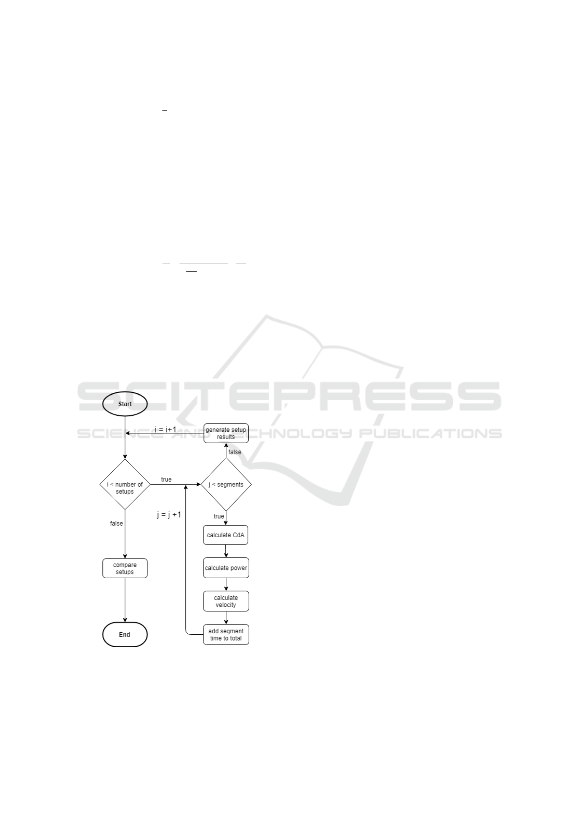
The logic of the simulation is illustrated in Figure 1,

where the total race time for each equipment setup and

the velocity proﬁle is calculated.

Figure 1: Flowchart showing how the model is used in a

discrete context.

The following assumptions are made.

Weather Conditions. The wind speed- and direction

are assumed to be constant for the whole simula-

tion, making V

w, j

and θ

the same for every seg-

ment. In reality, atmospheric wind will always

be turbulent over a large range of length scales.

Small scale turbulence can alter the ﬂow around

the cyclist compared to the low turbulent wind tun-

nel conditions. Large scale turbulence, also called

gustiness, will cause a instant shift in the C

A-

velocity-yaw set-point, and also, because of the

squared velocity dependency in the drag formula,

cause an underestimation of the simulated drag

force. Additionally, temperature and air pressure

are assumed constant for the whole simulation.

Turns and Braking. The model does not account for

braking and accelerating in and out of corners.

Brake patterns and turning technique varies from

corner to corner and rider to rider, thus no general

equation was implemented for this.

Power Input from Rider. Power input from the rider

is intended to be estimated from previous race data

as a function of road gradient. It is therefore as-

sumed that the rider will be able to deliver the same

power as deﬁned in the power-gradient curve.

2.2 Wind Tunnel Measurements

Wind tunnel measurements of two test riders were per-

formed in the wind tunnel at the Norwegian university

of science and technology (NTNU) in Trondheim. The

wind tunnel has a test section cross-section of 2.7 x

1.8 meters (w x h) and the resulting blockage ratio was

> 10 %. A blockage correction factor based on CFD

simulations was applied to the measured data. A time

trial bike was ﬁxed to a 6-component force balance

(Carl Schenck AG) supported by aerodynamic struts on

the fork and a bike trainer (Tacx Bushido) on the rear

hub. The free stream wind speed was measured with a

pitot-static tube, and the incoming wind speed was cor-

rected with the cosine of the yaw-angle for the yawed

test cases.

A comfortable time-trial position that could be

replicated in a ﬁeld test was chosen by each rider and

the drag force along the bike axis was measured with

the rider pedaling at a steady cadence. The inﬂuence of

variation in cadence on aerodynamic drag was investi-

gated and found to be negligible. The drag of the bike

support was also measured and subtracted from the to-

tal drag. Due to the inherent uncertainty related to rider

position and pedaling, 3 measurements of 20 seconds

sampling time were made and averaged for each test

case. A visual feedback system, including a side view

camera and overlaid guide lines, was installed in the

wind tunnel in order to aid the test riders maintain the

same position for all test cases.

icSPORTS 2019 - 7th International Conference on Sport Sciences Research and Technology Support

The drag area of the full rider and bike setup was

measured at 5 different wind speeds ranging from 30

km/h to 70 km/h, and at 4 different yaw angles rang-

ing from 0 to 15 degrees. The resulting data-set cov-

ers the conditions most commonly experienced during

a ﬂat time-trial. Drag values for simulated cases falling

outside of the measured data-set are set to the closest

measured value, but these cases are expected to be few

under normal race conditions.

2.3 Model Validation

2.3.1 Determination of Coefﬁcients

The moment of inertia of the wheels, the rotational drag

coefﬁcient of the wheels as well as power loss in wheel

bearings and chains were taken directly from (Martin

et al., 1998). The coefﬁcient of rolling resistance was

retrieved from (XBits, 2016) for a tire model similar

to the one used on the test bike. The values are listed

below.

Moment of inertia of wheels: I = 0.14kg · m

Rotational drag coefﬁcient: F

= 0.0044

Mechanical loss coefﬁcient: E

= 0.976

Coefﬁcient of rolling resistance: C

= 0.00297

2.3.2 Field Test

Validation of the model’s accuracy was done by con-

ducting tests on a 6.8km course with both ﬂat, uphill

and downhill sections. The C

A data-sets for the two

test riders from the wind tunnel was used in the sim-

ulations. Wind velocity and -direction, and tempera-

ture were measured on site, and the air pressure was

retrieved from the weather forecast of the day. Two

different test cases were chosen for each of the two test

riders, rider 1 testing two different skinsuits and rider

2 testing two different riding positions. The two riders

used the same TT-bike and -helmet. Total system mass

of the test riders and equipment was measured prior to

the test, as listed below.

Rider 1, Skinsuit 1: 92.9 kg

Rider 1, Skinsuit 2: 92.7 kg

Rider 2, Skinsuit 1: 92.7 kg

The course was ridden in both directions; south-

ward with 90m of climbing, and northwards with 19m

of climbing. Both with a net elevation gain and loss

of 72m respectively. The tests were done with a ﬂying

start of 8.5m/s southwards and 12.5m/s northwards.

Test rider 1 rode four tests; both directions with two

different skinsuits. Test rider 2 did two tests south-

wards with Skinsuit 1; once seated in an aerodynamic

time trial position and one standing up in hills inclined

by more than 4%. The bike was equipped with a crank

arm based power meter (Stages Cycling LLC), allow-

ing the riders to pace their power output during the

test. The riders were instructed to follow the simulated

power curve shown in Figure 2.

Figure 2: Power curve used in the simulation and measured

power for Test rider 1 in Test 1.

The power output for 0% incline was set to 250W

with an increase of power per % increase in gradient of

3.2W . Elapsed time, velocity and gradient were mea-

sured with a Garmin Edge®820 bike computer as well

as two independent stopwatches.

The wind conditions varied along the course during

the ﬁeld test. The northernmost 2.43km of the course

were exposed to wind while the remaining parts were

calm because of the surrounding terrain. Therefore, the

course was divided into a northern and southern sec-

tion, and the test was simulated in two steps; with wind

on the northern section, and with zero wind on the rest.

The two simulations were then merged. Additionally,

the simulations were run with both variable and con-

stant drag area, where the constant drag area was taken

from the average velocity of the test and zero yaw.

2.4 Subdivisions of Track Segments

A series of simulations of the southbound track was

done for Test rider 1 with Skinsuit 1 to ﬁnd a reso-

lution of segments that yields stable results. Simula-

tions were done with a wind of 0m/s, and tested with

2, 5, 10, 20, 40, 80, 160, 320, 640 and 1280 subdivi-

sions of the segments. The default resolution from the

GPS-tracker used is 1s. Table 1 below shows simula-

tions with the corresponding total simulation time for

the different subdivisions.

From the convergence in the graph observed in the

table, as well as illustrated in Figure 3, it can be as-

sumed that the result from simulations will not change

for simulations with more than 1280 sub-segments.

From this, a simulation with 1280 sub-segments can

be deﬁned as virtually accurate. An expression can

then be made for the relative simulation error with n

sub-segments as e

,rel

−v

1280

, where v

1280

is the es-

Simulation Model for Road Cycling Time Trials with a Non-constant Drag Area

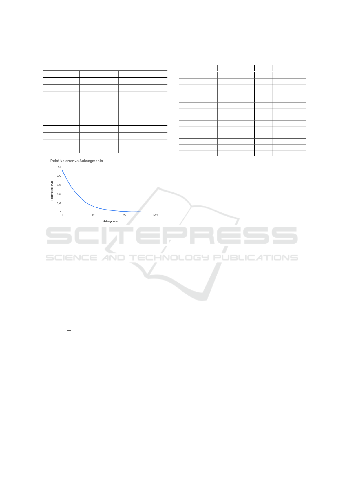
Table 1: Simulations of the southbound track for Test rider

1 with Skinsuit 1, wind velocity 0m/s.

Subdivisions Avg. Velocity Computation time

1 8.820 m/s 0.25 s

2 8.783 m/s 0.5 s

5 8.753 m/s 1.25 s

10 8.741 m/s 2.5 s

20 8.735 m/s 5 s

40 8.732 m/s 10 s

80 8.730 m/s 20 s

160 8.729 m/s 40 s

320 8.729 m/s 80 s

640 8.728 m/s 160 s

1280 8.728 m/s 320 s

Figure 3: Relative simulation error of average velocity vs.

number of sub-segments.

timated average velocity from the simulation with 1280

sub-segments.

Figure 3 shows that the relative error in simulation

decreases with an increase in subdivisions, and that the

results of the simulations converges monotonically. As

shown in Table 1, the simulation time increases with

the number of subdivisions. Therefore it is not desir-

able to choose a very high number of divisions, as the

gain in accuracy will be minimal compared to compu-

tational cost. The relative error for 40 sub-segments is

calculated to 0.05%, with an acceptable total computa-

tion time of approximately 10 seconds. Based on this,

a segment subdivision of 40, resulting in a segment res-

olution of

s, was chosen for the simulations.

3 RESULTS

The results of the validation test are summarized in Ta-

ble 2.

The mean absolute difference of the simulations is

3.22%. In Table 2, the symbols are deﬁned as shown

below.

R: Test rider

S: Skinsuit

D: Direction of the test course

Table 2: Results of model validation.

Test 1 2 3 4 5 6

R 1 1 1 1 2 2

S 1 1 2 2 1 1

D S N S N S S

S 0 0 0 0 0 0

N 3.5 2 2 2 1 1

dir

NE N-NE N-NW N-NW N N

T 15 15 15 15 17 17

p 1018 1018 1018 1018 1018 1018

P 254 245 254 244 265 261

MAE

22.0 20.2 19.2 23.5 43.0 39.7

12:21 9:23 12:35 9:28 12:02 12:24

11:58 9:08 12:29 9:04 12:41 12:46

-3.2% -2.7% -0.82% -4.3% 5.4% 2.9%

11:59 09:10 12:32 9:07 12:44 12:49

S: Wind velocity in the southern section [m/s]

N: Wind velocity in the northern section [m/s]

dir

: Wind direction [orientation]

T: Temperature [

◦

p: Air pressure [hPa]

P: Average power [W]

MAE

: Mean absolute error of power [W]

: Measured time [min : sec]

: Simulated time [min : sec]

: Relative error between t

and t

: Simulated time for a constant C

A [min : sec]

In Test 5 the time-trial position is retained through-

out the course, while in test 6 the rider used a standing

up position where the gradient exceeded 4%.

Figure 4, 5 and 6 shows the simulated velocity

plotted against the measured velocity along the test

course, in the southward direction. During the tests,

a delay in the gradient measured by the bike computer

was observed, meaning that when the gradient changes

quickly, such as in transitions into hills or over hilltops,

the measured gradient lags behind the terrain. This will

result in unrealistic simulated velocities on these sec-

tions of the course. Figure 5 also shows a drop in the

simulated velocity just before 1000 m. This is due to

the bike computer measuring a false gradient of 4-5%

over a short period at this point. Due to this, the drop

in velocity only shows up in the simulation and not in

the measured velocity.

4 DISCUSSION

As shown in Table 2, the simulated results deviate from

the actual time by 0.8%-5.4%. There are primarily

two sets of limitations that account for this deviation.

icSPORTS 2019 - 7th International Conference on Sport Sciences Research and Technology Support

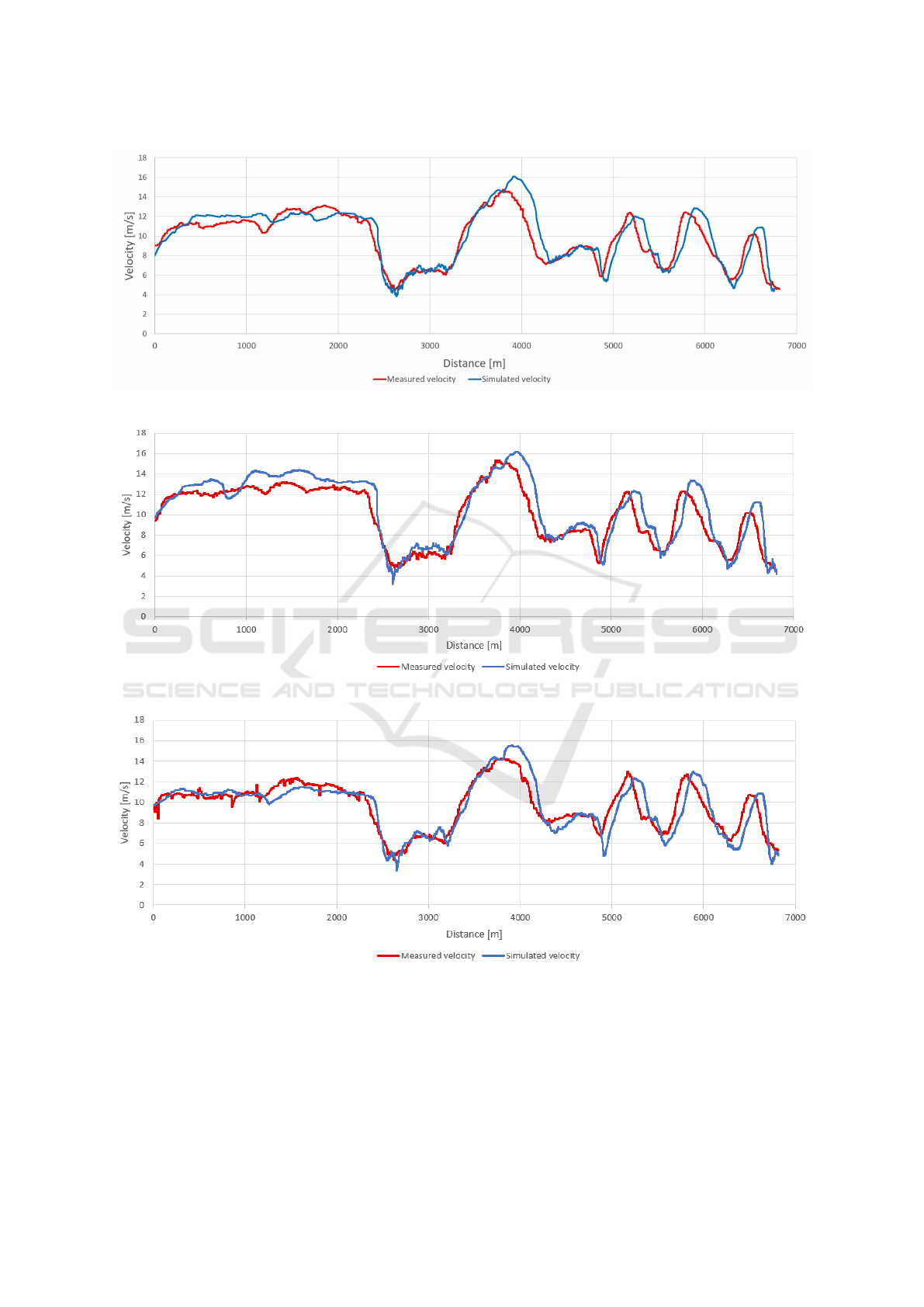
Figure 4: Simulated vs. measured velocity. Test rider 1, Skinsuit 2.

Figure 5: Simulated vs. measured velocity. Test rider 1, Skinsuit 1.

Figure 6: Simulated vs. measured velocity. Test rider 2, Skinsuit 1, standing position on hills.

One is the limitations of assumptions and simpliﬁca-

tions that are made for the model. As mentioned in

Chapter 2.3.1, values for the coefﬁcients for inertia in

the wheels, rotational drag of the wheels, mechanical

loss in wheel bearings and chains and rolling resistance

were retrieved from previous experiments by other au-

thors. Ideally these coefﬁcients should have been mea-

sured for the actual setup used in the test. This uncer-

tainty could have various effects on the results. Fur-

thermore, wind speed and direction are assumed to be

constant for a full simulation. This involves a simpli-

ﬁcation of the actual test conditions, as some of the

test runs were susceptible to changes in wind. It was

however possible to limit this uncertainty by running

Simulation Model for Road Cycling Time Trials with a Non-constant Drag Area

separate simulations, dividing the course into two sec-

tions with clear difference in wind conditions. The

model does not consider braking and cornering, and

this can lead to an underestimation of simulated time

for courses with fast downhill sections and sharp turns.

The other set of limitations is the data input to the

model. The wind tunnel data were measured for the

head down position that a rider normally uses during

straight sections of the course, where much attention

to the road ahead is not needed. In the validation tests

as well as in a race, this will not always be possible, as

curves and uneven road surfaces forces the rider to raise

their head to scan the road ahead. This will cause the

simulated time to be lower than the real time at certain

points. However, the time spent in the aero-position

increases with the level of the cyclist and is large com-

pared to the time spent in deviating positions for most

races. It is shown by (Olds et al., 1995) that riders of

a higher level also have a higher discipline of pacing

and positioning while riding. As none of the test rid-

ers hold international level as cyclists, this effect of

this will be greater in the performed tests than for a

World Tour rider. Wind tunnel tests were conducted

for no lower than 8m/s and no greater than 20m/s. The

drag area was assumed constant for any velocities be-

low 8m/s and over 20m/s in the simulations. The va-

lidity of the assumption of a constant drag area is de-

pendant on equipment and position, but the drag area

is more likely to increase slightly for lower velocities

based on the trend in wind tunnel test results in the Ap-

pendix. Velocities below 8m/s were measured at some

points during climbs and this leads to an underestima-

tion of drag in these hills, thus slightly overestimating

the velocity in the simulation. Also a signiﬁcant uncer-

tainty is related to the instantaneous power produced

by the test rider. Even though the average power was

fairly consistent between test runs, a random variation

around the predeﬁned power curve must be expected.

The MAE

row in Table 2 shows that the mean average

error of power input ranged from 19.2 to 43 watts.

Also, the power-slope function developed for this

simulation was based on a small data set. Ideally, the

power functions should be based on personalized his-

torical performance data for similar race conditions and

duration. Another limiting factor of the power curve is

that it does not account for a third dimension, namely

the length of the race. The average power of a short

time trial is signiﬁcantly higher than that of a long time

trial, and the power curve should be scaled accordingly.

It is shown in Figure 4 that the simulated velocity

deviates the most from the measured velocity in sec-

tions where there is a transition between high and low

velocity, typically where the gradient changes quickly,

as over a crest and in the transition into a hill. A de-

lay was observed in the gradients recorded by the GPS

computer. Due to this delay the simulation will pro-

duce unrealistic values in such sections of terrain tran-

sition. This results in the simulated velocity curve hav-

ing close to the same shape as the measured velocity

curve, but being shifted slightly to the right. The effect

is visible from the 4000m mark and onward in Figure

4. More accurate altitude data of the course should lead

to more accurate simulations.

Because the wind conditions varied in between the

test runs, it is hard to determine with certainty that one

equipment setup is indeed faster than the other. The

trends observed in the measurements do however in-

dicate that Skinsuit 1 is superior to Skinsuit 2 while

riding the course in both directions. When simulating

both setups against each other with equal conditions,

Skinsuit 1 is predicted to be the faster one of the two.

Additionally, the wind tunnel tests results in the Ap-

pendix show that Skinsuit 1 gives a lower drag coefﬁ-

cient than Skinsuit 2. This indicates that the model is

able to predict which of the setups is the fastest.

In Table 2, results from simulations with a con-

stant drag area are included. Based on the wind tun-

nel tests results shown in the Appendix, the drag area

will vary with velocity (and Reynolds number). The

general tendency in these tests was that the predicted

time became slightly higher with a constant drag area.

It is believed that time trials spanning a greater velocity

interval will lead to greater differences between simu-

lations with or without a changing drag area. This will

also depend largely on the velocity proﬁle and shape

of the C

-velocity curve. For the two skinsuits tested

here, the shape of the C

-velocity curves do not inter-

sect and consequently Skinsuit 1 will give a higher ve-

locity throughout the course in both directions.

From the total of six tests that were conducted, the

mean absolute error of 3.22% was within the frame

of the objectives. Because of the low sample size, in

which every test was unique in form of a different rider,

equipment setup or course, there is not much basis to

name the statistical uncertainty of the simulations. Nor

are there enough empirical results to claim that this

model of prediction is any more accurate than previous

models. However, despite the difﬁculty of performing

accurate ﬁeld tests involving human test subjects, the

test results indicate that the fastest setup identiﬁed from

the wind tunnel tests, is also faster on the road. Also,

given accurate input data, the model should be able to

predict the fastest setup for otherwise similar race con-

ditions.

5 CONCLUSIONS

Based on the experiments conducted in this paper, the

expanded model for predicting road cycling perfor-

mance may be used to identify the best equipment setup

for any given time trial and rider. Simulations of the

conducted ﬁeld tests showed a mean absolute differ-

ence of 3.22%, which was within the range of previous

icSPORTS 2019 - 7th International Conference on Sport Sciences Research and Technology Support

studies. Further experiments and validation is required

to determine the statistical uncertainty of the model and

the sensitivity to the errors in the various input param-

eters.

ACKNOWLEDGEMENTS

We would like to express our gratitude to Team INEOS,

and Sondre Bergtun Auganæs of Centre for Sports Fa-

cilities and Technology at NTNU for their contribu-

tions and support throughout this project.

REFERENCES

Dahmen, T., Byshko, R., Saupe, D., R

oder, M., and

Mantler, S. (2011). Validation of a model and a simu-

lator for road cycling on real tracks. Sports Engineer-

ing, 14(2):95–110.

Dahmen, T. and Saupe, D. (2011). Calibration of a power-

speed-model for road cycling using real power and

height data. International Journal of Computer Sci-

ence in Sport, 10:18–36.

E di Prampero, P., Cortili, G., Mognoni, P., and Saibene,

F. (1979). Equation of motion of a cyclist. Journal

of applied physiology: respiratory, environmental and

exercise physiology, 47:201–6.

Martin, J. C., Milliken, D. L., Cobb, J. E., McFadden, K. L.,

and Coggan, A. R. (1998). Validation of a mathemati-

cal model for road cycling power. JOURNAL OF AP-

PLIED BIOMECHANICS, 14(3):276–291.

Olds, T., Norton, K. I., and Craig, N. O. (1993). Mathemat-

ical model of cycling performance. Journal of applied

physiology, 75(2):730–7.

Olds, T. S., Norton, K. I., Lowe, E. L., Olive, S., Reay,

F., and Ly, S. (1995). Modeling road-cycling perfor-

mance. Journal of Applied Physiology, 78(4):1596–

1611. PMID: 7615475.

XBits, J. B. (2016). Tire test - continental grand prix

tt. https://www.bicyclerollingresistance.com/road-

bike-reviews/continental-grand-prix-tt-2016. Ac-

cessed on 09/04/2019.

APPENDIX

Drag area vs. velocity for Test rider 1 with skinsuit 1 and 2.

Simulation Model for Road Cycling Time Trials with a Non-constant Drag Area