Improvement of Pairwise Comparison by using Response Time
Yoshiki Sakamoto
1
, Takashi Kurushima
1
, Kimi Ueda
1
, Hirotake Ishii
1
, Hiroshi Shimoda
1
,
Rika Mochizuki
2
and Masahiro Watanabe
2
1
Graduate School of Energy Science, Kyoto University, Yoshida-honmachi, Sakyo-ku, Kyoto, Japan
2
Organization of Service Evolution Laboratories, NTT Group, Hikarinooka, Yokosuka-shi, Kanagawa-ken, Japan
Keywords: Pairwise Comparison, Response Time, Correction Function.
Abstract:
Pairwise comparison has been widely employed as an easy method for subjective evaluation of several candi-
dates to develop new products or to improve service. In this paper, a method using response time was proposed
to improve the accuracy of pairwise comparison. Firstly, a pairwise comparison experiment was conducted to
investigate the relationship between response time and difficulty of judgement. Then, a method to improve the
accuracy of calculated scales of the objects was proposed where the answer of the pairwise comparison was
modified by using the response time and correction function. In this study, three correction functions were
compared to find the difference of the accuracy improvement, and two of them showed significant improve-
ment.
1 INTRODUCTION
These days, they have tried to improve products and
services based on “how people feel”(e.g., senses,
emotions, preference or comfort). This method in af-
fective evaluation is called “Kansei evaluation”. Kan-
sei evaluation has made it possible to find the needs
hidden in human senses in many industries.
There are various methods of Kansei evaluation.
Among them, pairwise comparison is widely used in
various fields. In pairwise comparison, two out of
several objects to be evaluated are presented and the
evaluator judges better one by comparing the pair. All
the combination of two objects are presented like this
and the preferable scale values of each object are cal-
culated based on the judgments. Pairwise compari-
son has the advantage that the evaluator’s burden is
light since only two objects are compared at a time
and a relative evaluation is required rather than an ab-
solute evaluation. Moreover, it is possible to quantify
not only the order of each object but also the scale
value. Nakae et al. used pairwise comparison to eval-
uate patients’ pain (Nakae et al., 2018). Francis et
al. used it to assess performance of judges from court
data (Francis et al., 2001).
There are some methods for pairwise compari-
son. Thurstone’s pairwise comparison method, which
judges only by superiority or inferiority between the
two stimuli, and Scheffe’s pairwise comparison
method, which judges by giving scores of the two,
are the typical examples. Thurstone’s pairwise com-
parison method is easy for the evaluator because it
requires an either-or decision, such as “Prefer the
left / Prefer the right”. On the other hand, Scheffe’s
pairwise comparison method requires multiple scores,
which has the advantage in its high accuracy and the
disadvantage that the judgment is complicated and the
burden on the evaluator is heavier. Furthermore, in re-
ality, there are many cases when the evaluator is dif-
ficult to make complicated judgments such as infants
or when it is only possible to collect binary data such
as winning and losing in sports (Usami, 2009).
For the above reasons, it is desirable to use the
Thurstone’s paired comparison method in considera-
tion of versatility. In the Thurstone’s pairwise com-
parison method, however, the obtained scale value al-
ways contains an error (Tabata et al., 1995).
In this study, the authors focus on the response
time to improve Thurstone’s pairwise comparison.
Since Thurstone’s pairwise comparison method re-
quires an either-or decision, the evaluator has to
choose one of the two options. In case that there is
an obvious difference between the two, the evalua-
tors answer with confidence and the obtained answer
is highly reliable. When the difference is not obvi-
ous, however, “hesitation” occurs in the evaluators,
104
Sakamoto, Y., Kurushima, T., Ueda, K., Ishii, H., Shimoda, H., Mochizuki, R. and Watanabe, M.
Improvement of Pairwise Comparison by using Response Time.
DOI: 10.5220/0008161801040111
In Proceedings of the 3rd International Conference on Computer-Human Interaction Research and Applications (CHIRA 2019), pages 104-111
ISBN: 978-989-758-376-6
Copyright
c
 2019 by SCITEPRESS – Science and Technology Publications, Lda. All rights reserved

and they answer without confidence, so the reliability
of the answer result may be low. Thus, assuming that
the reliability of the answer is high when the response
time is short while it is low when the response time
is long, if the relationship between the difficulty of
the comparison task and the response time is clarified
and the answer that takes the “hesitation” into account
can be obtained, it would be able to get high accurate
results regardless of the simplicity of the comparison
task.
2 CONVENTIONAL METHOD
2.1 Thurstone’s Paired Comparison
Method
Thurstone’s paired comparison method (Thurstone,
1927) is a method in which answers are made by two
alternatives. Now, a pair ( j, k) ( j, k = 1, 2, ··· , n) is
created from n stimuli. When let the evaluator choose
either j or k from the pair ( j, k), let p
jk
be the proba-
bility that j is chosen and x
jk
be the lower percentage
point of p
jk
. For each pair ( j, k), suppose that N in-
dependent comparisons were made. The scale values
S
D
( j) are expressed as
p
jk
=
1
√
2π
Z
∞
x
jk
exp(−
x
2
2
)dx (1)
∑
j
{x
jk
−S
D
(k) +S
D
( j)} = 0 (2)
Therefore,
S
D
(k) =
1
n
n
∑
j=1
x
jk
(3)
2.2 Gulliksen’s Method
As can be seen from Eq.(1), when p
jk
is 0 or 1, x
jk
becomes +∞ or −∞ respectively, and missing values
appear in the matrix X which has x
jk
as an element.
When a calculation method for such incomplete data,
there is the Gulliksen’s method (Gulliksen, 1956).
When X is an incomplete matrix, Eq.(2) is ex-
pressed as
n
k
∑
j
{x
jk
−S
D
(k) +S
D
( j)} = 0 (4)
n
k
is the number of x
jk
which exists in k columns of
X. Therefore, Eq.(4) gives the following: Eq.(5).
Z = M S (5)
Where,
Z =













n
1
∑
j
x
j1
n
2
∑
j
x
j2
.
.
.
n
n
∑
j
x
jn













(6)
S =




S
D
(1)
S
D
(2)
.
.
.
S
D
(n)




(7)
M is a n ×n symmetric matrix which has n
k
in its
main diagonal line, −1 when x
jk
exists and 0 when
the value misses. The origin of the scale S
D
, for exam-
aple, is defined as S
D
(1) = 0.
S
1
= M
−1
11
Z
1
(8)
S
1
and Z
1
are given by deleting the first element from
S and Z, and M
11
is given by deleting the first row
and the first column from M . By solving Eq.(8), the
value of S
D
(k)(k ≥2) with S
D
(1) as the origin can be
found.
3 PROPOSED METHOD
3.1 Outline
In the proposed method, the accuracy of the Thur-
stone’s pairwise comparison method, the closeness
between the obtained scale value and true value of the
evaluated object, will be improved by reflecting the
“hesitation” information obtained from the response
time.
A function that corrects the answer of the either-or
decision from the response time (hereinafter referred
to as “correction function”) is considered. In pairwise
comparison, when a stimulus pair ( j, k) is given and
stimulus j is selected, p
jk
= 1, p
k j
= 0. For exam-
ple, when using the answer result p and the response
time t, the correction function f corrects the answer
as below.
(p
jk
, p
k j
) = (1, 0) −→
f
(0.6, 0.4) (9)
3.2 Correction Function
In this study, three correction functions are proposed
to generate an optimal model. First, the conditions
Improvement of Pairwise Comparison by using Response Time
105

that the correction function should satisfy are listed
below.
In the Thurstone’s pairwise comparison method,
the evaluator has to select either one of the two pre-
sented options, giving
p
jk
+ p
k j
= 1 (10)
p ∈ {0, 1} (11)
Assuming that the correction function f (p,t) is a
function where inputs the answer result p and the re-
sponse time t, and the output is a modified probability.
f (p
jk
,t) + f (p
k j
,t) = 1 (12)
0 ≤ f (p, t) ≤ 1 (13)
Assume that the superiority of the answer result is not
reversed.
f (0, t) ≤ f (1,t) (14)
Assume that the answer result p converges to 0.5
when the answer time increases.







∂ f (1,t)
∂t
≤ 0
∂ f (0,t)
∂t
≥ 0
(15)
lim
t→∞
f (p,t) = 0.5 (16)
The following “Correction function 1” and “Cor-
rection function 2” are created as candidates that sat-
isfy from Eq. (10) to Eq. (16) and may improve the
accuracy of the pairwise comparison.
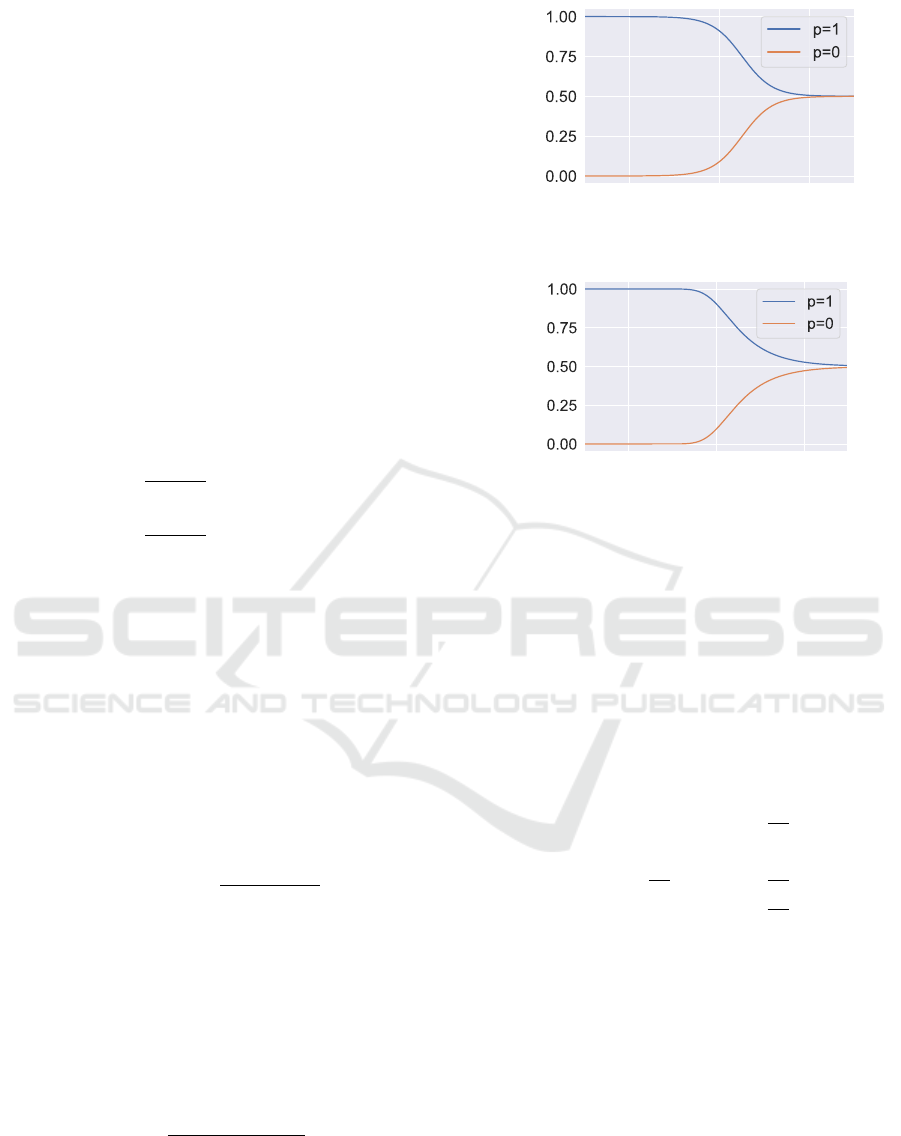
3.2.1 Correction Function 1
The following correction function 1: f
1
(p, t) is de-
fined. The outline of correction function 1 is shown
in Fig.1. x
0
and x
1
are the parameters of the function.
f
1
(p, t) = g
1
(t) ·(p −0.5) + 0.5 (17)
g
1
(t) =
1
1 + e
x
0
·(t−x
1
)
(18)
From Eq. (15)
x
0
> 0 (19)
3.2.2 Correction Function 2
The following correction function 2: f
2
(p, t) is de-
fined. The outline of correction function 2 is shown
in Fig.2. x
0
and x
1
are the parameters of the function.
f
2
(p, t) =
1
1 + e
−g
2
(t)·(p−0.5)
(20)
g
2
(t) = e
−x
0
·(t−x
1
)
(21)
From Eq. (15)
x
0
> 0 (22)
t 
f(p,t)

Figure 1: Correction Function 1.
t 
f(p,t)

Figure 2: Correction Function 2.
3.2.3 Correction Function 3
In the physiological field, linear regression is often
applied as a method with high generalization perfor-
mance (Picard et al., 2001; Kunimasa et al., 2017).
Thus, the following correction function 3: f
3
(p, t) is
defined. The outline of correction function 3 is shown
in Fig.3.
f
3
(p, t) = g
3
(t) ·(p −0.5) + 0.5 (23)
g
3
(t) =









1 (t < −
1
2x
0
+ x
1
)
−x
0
·(t −x1) + 0.5
(−
1
2x
0
+ x
1
≤t <
1
2x
0
+ x
1
)
0 (t ≥
1
2x
0
+ x
1
)
(24)
From Eq. (15)
x
0
> 0 (25)
By applying the correction function to the ob-
tained answer result matrix p = (p
jk
) and the re-
sponse time matrix t = (t
jk
) , the modified result ma-
trix f= ( f (p
jk
,t
jk
)) is created. Then, the scale value
of each stimulus is calculated using the Gurriksen
method described in Section 2.2.
3.3 Accuracy Evaluation Method
To evaluate the proposed method, the scale value of
each stimulus is compared with the actual physical
CHIRA 2019 - 3rd International Conference on Computer-Human Interaction Research and Applications
106

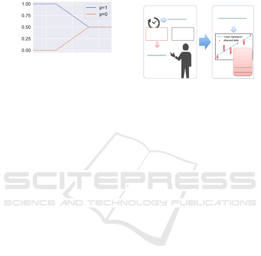
t 
f(p,t)

Figure 3: Correction Function 3.
quantity of the stimulus. The stimulus to be used for
the accuracy evaluation should be, therefore, quantita-
tively measured such as brightness, sound volume and
length of object. When the calculated scale value of
each stimulus and the physical quantity of each stim-
ulus are in a linear relationship, the coefficient of de-
termination could be used to evaluate the accuracy of
the scale values. That is, simple regression analysis is
performed using the physical quantity (e.g. tempera-
ture, length, weight) of each stimulus as the explana-
tory variable and the scale value as the objective vari-
able, and the coefficient of determination R
2
is calcu-
lated from the simple regression equation. The closer
the coefficient of determination R
2
is to 1, the more
accurate is the scale value.
3.4 Accuracy Improvement Method in
Pairwise Comparison
The outline of the accuracy improvement method in
this study is shown in Fig.4. First, from the modified
result matrix f = ( f (p
jk
,t
jk
)) obtained by applying
to the correction function, the scale values is calcu-
lated by the method of Gurriksen described in Section
2.2. Then, using x
0
and x
1
of the correction function
described in Section 3.2 as variables, the correction
function can be optimized to maximize the coefficient
of determination R
2
by adjusting the parameters such
as x
0
and x
1
. If the same stimulus pair is compared
multiple times, the average value of f (p
jk
,t
jk
) is used
for scaling.
The differential evolution method which is a
global optimization method of evolutionary algorithm
(Storn and Price, 1997) is adopted for optimization
of the correction functions. By optimizing x
0
and
x
1
where the coefficient of determination R
2
is max-
imized, a correction function can be determined that
improves the accuracy of the scale.
k  j 
Response'time''
matrix
t=(t
jk
)
p=(p
jk
)
Answer'result'
matrix
Pairwise'comparison'task
f=(f(p
jk
,t
jk
))
Modified'result'
matrix
f 
Correction''
function'
Scale'value'
Optimize'
correction'
Function'
'
'

max.'''R
2)
's.t.'''x
0
,'x
1
'
'
Figure 4: Accuracy Improvement Method.
4 EVALUATION EXPERIMENT
In this study, the relationship between the difficulty
of the comparison and the response time was firstly
confirmed, then the accuracy improvement of the pro-
posed method was evaluated.
4.1 Participants
Twenty-eight male students participated in the exper-
iments. All participants had normal or corrected-to-
normal vision confirmed by taking a questionnaire.
Their average age was 21.4 (SD = 2.0).
4.2 Task
The outline of the task used in this experiment is
shown in Fig.5, and the actual graphical interface of
the task is shown in Fig.6 . In this experiment, a pair-
wise comparison task was created in which two lines
were displayed side by side as the stimuli and the par-
ticipants were asked to answer the longer one.
The reason to adopt the pairwise comparison task
which asks the length of the line is as follows; first,
the smaller the difference between the actual lengths
of the two presented lines, the higher is the task diffi-
culty, and it is possible to quantitatively estimate the
task’s difficulty, that is, the tendency to hesitation.
Another reason is that line length is hardly affected by
the experimental environment. For example, in com-
parison of color, the degree of difficulty can be quanti-
tatively evaluated from the distance in color map, but
how to feel the stimulus is greatly influenced by such
as the brightness of the display and the illumination
of the experimental room.
In this experiment, six lengths of vertical lines
(200px, 202px, 204px, 206px, 208px, 210px) were
used as comparison stimuli. The actual lengths on the
display were 50.0 mm, 50.5 mm, 51.0 mm, 51.5 mm,
Improvement of Pairwise Comparison by using Response Time
107

52.0 mm, and 52.5 mm, respectively. The distance
between the participant and the display was 0.80 m,
and the calculated viewing angles were about 3.58
◦
,
3.62
◦
, 3.65
◦
, 3.69
◦
, 3.72
◦
and 3.76
◦
, respectively.
The widths of the line were all 3 px.
START
+
FINISH
+
Gaze%point%
3%sec.
Gaze%point%
6-t%sec.
Comparison%task%
t%sec.
*%0%≦%t%≦%4.0%sec.%
6%sec.%×%36%trials%
Figure 5: Outline of the task.
Figure 6: The actual graphical interface of the task (com-
parison task).
Two of the vertical lines as comparison stimuli
were displayed side by side, and 36 pairs, including
pairs of the same length were presented. A series of
tasks comparing all the 36 pairs was called one set. A
gaze point was displayed at the center every time the
pair was switched to make the participant’s gaze in
the center of the display. The response was input by
clicking on the button displayed under the line which
the participant felt longer. The time from the presen-
tation of the pair to the response was measured. If
there was no response within 4.0 seconds, the presen-
tation of the pair was automatically terminated and
the gaze point was displayed.
4.3 Experiment Environment
The participants were asked to use a computer mouse
to conduct the pair comparison task displayed on the
screen. The screen size of the display (I-O DATA,
LCD-MF243EBR) was 23.6 inches, and the resolu-
tion was 1920 × 1080. The illuminance on the desk
was 330 lx.
Response'
time
long
short
200
200202204 206 208210
202
204
206
208
210
Length'(left)'
Length'(right)'
Figure 7: Result of all participants (average).
4.4 Experimental Procedure
The experiment was conducted in the period of Jan-
uary 4th to 19th, 2019. All the participants performed
a practice of the comparison test for about one minute
before the experiment. After that, 12 sets of the tasks
described in Section 4.2 were done. A 3 minute break
was provided between each set.
4.5 Results
In this experiment, the participants who did not an-
swer within the time limit more than 36 times among
the 12 sets / 432 trials, or who selected one of the left
and right sides more than 360 times out of 432 trials
were considered not to be seriously engaged in the ex-
periment, and were excluded from the analysis below
as invalid data. In addition, comparisons that was not
answered within 4.0 seconds were regarded as invalid
data and were excluded from the analysis.
The average response time of all the participants
for each stimulus pair is shown in Fig.7. The verti-
cal axis indicates the line length in pixel displayed on
the left side, while the horizontal axis indicates that
on the right side. The lighter the color in the cell, the
longer is the response time. The response time was
standardized for each set to reduce the variation in re-
sponse time for each experiment participant and each
set.
As a result, it was confirmed that the average re-
sponse time for the all participants tends to increase
as the difference in the length decreases.
Next, the results of each participant are described.
Here too, the response time was standardized for each
set in order to reduce the variation in the response
time. As an example of the results, the average re-
sponse time of all sets of participant number 10 is
shown in Fig.8. It was confirmed that the response
time tends to increase as the difference in the length
decreases. On the other hand, as the response answer
time of all sets of participant number 24 shown in
CHIRA 2019 - 3rd International Conference on Computer-Human Interaction Research and Applications
108

Response'
time
long
short
200
200202204 206 208210
202
204
206
208
210
Length'(left)'
Length'(right)'
Figure 8: Result of participant no.10.
Fig.9, there were no such tendency in some partici-
pants.
Response'
time
long
short
200
200202204 206 208210
202
204
206
208
210
Length'(left)'
Length'(right)'
Response'
time
long
short
200
200202204 206 208210
202
204
206
208
210
Length'(left)'
Length'(right)'
Figure 9: Result of all participant no.24.
5 EVALUATION OF THE
PROPOSED METHOD
In this chapter, the accuracy improvement effect of the
proposed method described in Chapter 3 is evaluated
using the answer results and response time measured
in the experiment.
5.1 Evaluation Method for the Proposed
Method
First, the answer result and the response time of learn-
ing data were applied to each correction function, and
the correction function was optimized to maximize
the coefficient of determination R
2
for each partici-
pant. The optimized correction function was created
by the method described in chapter 3. After that, the
accuracy improvement effect of the proposed method
was evaluated using test data.
Cross validation was used to evaluate the per-
formance of the optimized correction function. The
cross validation is a method of evaluating the accu-
racy of a model by applying one of the measurement
data divided into K as test data and the rest as training
data.
In this study, 12 sets performed by each partici-
pant were divided into four and the optimized correc-
tion function was created from the training data of the
9 sets. After that, the remaining 3 sets were applied
to the optimized correction function, and the accuracy
was evaluated by calculating the coefficient of deter-
mination R
2
. Finally, the coefficient of determination
R
2
of each of the four divisions was calculated, and
the average value was taken as the estimated accuracy
of the participant.
The data of participant number 5 and 18 were
treated as invalid data for the reason described in Sec-
tion 4.4. In addition, for 3 participants in the partici-
pant number 7, 9 and 14, there were too many missing
values in the answer results in some test data that M
11
in equation (8) has become a singular matrix with no
inverse matrix. Therefore, the scale value could not
be calculated and was excluded from analysis.
Python’s open source machine learning library
“scikit-learn” (sci, 2019) was used to calculate the co-
efficient of determination, and the “differential evo-
lution” function in Python’s open source numerical
calculation library “SciPy” (Sci, 2018) was used to
optimize the correction function.
5.2 Evaluation Results of the Proposed
Method
With regard to the correction function 1, the average
of the estimated accuracy of all the participants be-
fore the function was applied was 0.849, and that af-
ter the function was applied was 0.907. As a result
of paired t-test before and after applying correction
function 1, there was a significant difference at 1%
level (p = 0.00184 < 0.01).
With regard to the correction function 2, the av-
erage of the estimated accuracy of all the participants
before the function was applied was 0.849, and that
after the function was applied was 0.914. As a result
of paired t-test before and after applying correction
function 2, there was a significant difference at 0.1%
level (p = 0.000740 < 0.001).
With regard to the correction function 3, the av-
erage of the estimated accuracy of all the participants
before the function was applied was 0.849, and that
after the function was applied was 0.883. As a re-
sult of paired t-test before and after applying correc-
tion function 3, there was no significant difference
(p = 0.0526).
5.3 Discussion
First, participant number 24 is considered whose esti-
mated accuracy has decreased for all correction func-
Improvement of Pairwise Comparison by using Response Time
109

tions. As shown in Fig.9, the accuracy decreased be-
cause the response time did not tend to increase as the
difference in the length decreased. It was not consis-
tent with the assumption when creating the correction
function that “when the evaluator’s response time is
short, confidence in the answer is high, and when the
evaluator’s response time is long, confidence in the
answer is low”. On the other hand, as shown in Fig.8,
the accuracy in participant number 10 increased be-
cause the response time tended to increase as the dif-
ference in the length decreased.
Then, the result of participant number 26 is dis-
cussed. Table 1 to 3 shows the values of the parame-
ters in each test data, the scale value after applying the
correction function, the coefficient of determination
R
2
before applying the correction function, and the
coefficient of determination R
2
after applying the cor-
rection function. No significant difference was found
in the coefficient of determination R
2
between the cor-
rection functions for iteration number 1 to 3 after ap-
plying the correction function. This is because x
0
, the
gradient of the correction function, takes a value close
to 0 in all correction functions. At this time, from Eq.
(17) to Eq. (25), each correction function does not re-
flect the response time data, and the coefficient of de-
termination R
2
after applying the correction function
takes a value close to the coefficient of determination
R
2
before applying the correction function. For iter-
ation number 4, the coefficient of determination R
2
decreased after applying the correction function. This
is because x
0
was large and x
1
was small in correction
function 1 and correction function 3. Since the cor-
rection function is close to 0.5 for the answer with a
long response time, it loses high-precision data before
applying the correction function.
Table 1: Results (correction function 1, participant number
26).
iteration x
0
x
1
R
2
R
2
number (before) (after)
1 0.294 1.463 0.963 0.941
2 0.000 -2.076 0.862 0.943
3 0.000 -2.997 0.953 0.967
4 2.725 -1.471 0.921 0.768
Finally, the result of participant number 22 is dis-
cussed as shown in Table 4 to 6. No significant dif-
ference was found between the correction functions
for iteration number 1, 3, and 4. For iteration num-
ber 2, however, the coefficient of determination R
2
decreased only in correction function 3. At iteration
number 2, the coefficient of determination before ap-
plying the correction function was low, and the error
due to the answer itself was large. In the correction
function 1 and 2, however, the value of x
1
is extremely
Table 2: Results (correction function 2, participant number
26).
iteration x
0
x
1
R
2
R
2
number (before) (after)
1 0.185 3.000 0.963 0.935
2 0.000 -1.524 0.862 0.942
3 0.000 2.620 0.953 0.967
4 0.000 -0.672 0.921 0.993
Table 3: Results (correction function 3, participant number
26).
iteration x
0
x
1
R
2
R
2
number (before) (after)
1 0.073 1.000 0.963 0.939
2 0.000 0.486 0.862 0.943
3 0.000 0.572 0.953 0.967
4 4.590 -0.869 0.921 0.618
small, and from Eq. (17) to Eq.(22), the correction
function is always close to 0.5 regardless of the re-
sponse time and response result, so the original low
coefficient of determination improved. On the other
hand, since the value of x
1
is relatively large in cor-
rection function 3, it is strongly influenced by the low
original coefficient of determination.
Table 4: Results (correction function 1, participant number
22).
iteration x
0
x
1
R
2
R
2
number (before) (after)
1 3.000 0.261 0.962 0.927
2 0.393 -3.000 0.659 0.913
3 0.562 -3.000 0.450 0.960
4 3.000 -0.230 0.940 0.950
6 CONCLUSIONS
In this study, response time was applied to pairwise
comparison to improve the accuracy of it.
First, the response time was measured by an ex-
periment through a pairwise comparison task, and the
relationship between the difficulty of the comparison
and the response time was investigated. In this ex-
periment, a pairwise comparison task was created in
which two lines were displayed side by side and the
participants were asked to answer the longer one. As
the result, when averaged across the participants, the
response time tended to increase as the difference in
length decreased. In addition, when the participants
were examined individually, the same tendency was
also observed in some participants.
Next three types of “correction function” were
created to improve the accuracy of the pairwise com-
CHIRA 2019 - 3rd International Conference on Computer-Human Interaction Research and Applications
110

Table 5: Results (correction function 2, participant number
22).
iteration x
0
x
1
R
2
R
2
number (before) (after)
1 0.421 -3.000 0.962 0.952
2 0.264 -3.000 0.659 0.911
3 0.448 -3.000 0.450 0.960
4 0.450 -3.000 0.940 0.973
Table 6: Results (correction function 3, participant number
22).
iteration x
0
x
1
R
2
R
2
number (before) (after)
1 5.000 -0.296 0.962 0.953
2 5.000 0.432 0.659 0.468
3 4.985 0.309 0.450 0.934
4 4.987 -0.354 0.940 0.970
parison method. They modified the answered results
from the response time based on the above idea. As
the result, the accuracy improved significantly in two
correction functions.
In this study, a pairwise comparison task asking
the length of the line was used. However, only one
type of pairwise comparison task was investigated,
and it could not be asserted that the accuracy of the
pairwise comparison method always improved from
the result of this study. It is necessary to make more
pair comparison tasks with more modalities and to
conduct experiments and investigations to put the pro-
posed method into practical use. In addition, although
three types of correction functions were proposed in
this study, it is necessary to find more appropriate cor-
rection functions.
REFERENCES
(Dec 17, 2018). Scipy website. https://docs.scipy.
org/doc/scipy/reference/generated/scipy.optimize.
differential
evolution.html.
(Jan 31, 2019). scikit-learn website. https://scikit-learn.org/
stable/.
Francis, B., Soothill, K., and Dittrich, R. (2001). A new
approach for ranking ‘serious’ offences. the use of
paired-comparisons methodology. The British Jour-
nal of Criminology, 41(4):726–737.
Gulliksen, H. (1956). A least squares solution for paired
comparisons with incomplete data. Psychometrika,
21(2):125–134.
Kunimasa, S., Seo, K., Shimoda, H., and Ishii, H. (2017).
An estimation method of intellectual work perfor-
mance by using physiological indices. 6th Annual In-
ternational Conference on Cognitive and Behavioral
Psychology.
Nakae, A., Soshi, T., Tsugita, Y., Kishimoto, C., and Kato,
K. (2018). Objective evaluation of pain using experi-
mental heat stimulation. PAIN RESEARCH, 33(1):40–
46.
Picard, R. W., Vyzas, E., and Healey, J. (2001). Toward
machine emotional intelligence: Analysis of affec-
tive physiological state. IEEE Transactions on Pat-
tern Analysis and Machine Intelligence, 23(10):1175–
1191.
Storn, R. and Price, K. (1997). Differential evolution - a
simple and efficient adaptive scheme for global opti-
mization over continuous spaces. Journal of Global
Optimization, 11:341–359.
Tabata, Y., Ohga, Y., Kakuta, M., Nakamae, M., Morioka,
M., Uto, F., Okunisi, T., Oti, T., and Maeda, K. (1995).
Confidence coefficient of subjective scale value in
method of paired comparisons (case v). Japanese So-
ciety of Radiological Technology, 51(4):445–449.
Thurstone, L. L. (1927). The method of paired comparisons
for social values. Journal of Abnormal & Social Psy-
chology, 21(4):384–400.
Usami, S. (2009). Analyzing paired-comparison data in the
situation where judgment is affected by multiple fac-
tors. Japanese Psychological Research”, 79(6):536–
541.
Improvement of Pairwise Comparison by using Response Time
111