A Comparison of A* and RRT* Algorithms with Dynamic and Real Time

Constraint Scenarios for Mobile Robots

ao Braun

1 a

, Thadeu Brito

2 b

, Jos

e Lima

3,4 c

, Paulo Costa

3 d

, Pedro Costa

3 e

and Alberto Nakano

1 f

Federal University of Technology - Paran

a, Toledo, Brazil

CeDRI - Research Centre in Digitalization and Intelligent Robotics, Portugal

INESC TEC - INESC Technology and Science, Faculty of Engineering of University of Porto, Portugal

CeDRI - Research Centre in Digitalization and Intelligent Robotics, Polytechnic Institute of Braganc¸a, Portugal

Keywords:

Mobile Robotics, Path Planning, A-Star, RRT-Star, Dynamics Simulation.

Abstract:

There is an increasing number of mobile robot applications. The demanding of the Industry 4.0 pushes the

robotic areas in the direction of the decision. The autonomous robots should actually decide the path according

to the dynamic environment. In some cases, time requirements must also be attended and require fast path

planning methods. This paper addresses a comparison between well-known path planning methods using a

realistic simulator that handles the dynamic properties of robot models including sensors. The methodology

is implemented in SimTwo that allows to compare the A* and RRT* algorithms in different scenarios with

dynamic and real time constraint scenarios.

1 INTRODUCTION

In the last decades the planning of movements has

attracted much attention from the academic and in-

dustrial sectors. Generally, the main goal is to al-

low mobile robots to run their own movements au-

tonomously. The sensing, together with the imple-

mentation of algorithms, assists the execution of these

tasks. However, for many of the situations, only join-

ing these two tools does not make the drive of the

robot so trivial.

The task becomes even more arduous when one

considers the actions of the physical laws applied dur-

ing the trajectory of the robot. Even the design, the

disposition of the environment and the task that the

robot will perform, inﬂuence the ﬁnal result of the

autonomous movement. In this respect, trying to de-

velop a solution for any robot conﬁguration and at the

same time dealing with any physical eventualities, is

of great value for the execution of the robotic appli-

https://orcid.org/0000-0003-0276-4314

https://orcid.org/0000-0002-5962-0517

https://orcid.org/0000-0001-7902-1207

https://orcid.org/0000-0002-4846-271X

https://orcid.org/0000-0002-0435-8419

https://orcid.org/0000-0002-3757-1427

cation (Choset et al., 2005). The importance of auto-

matic motion planning goes beyond the need to make

a mobile robot capable of calculating its own path.

The possibility of transforming the process into dy-

namic situations results in a wide range of new tasks,

such as avoiding obstacles in the trajectory while the

robot is already moving.

In this way, the objective of this work is to com-

pare the performance of two path planning algorithms

when considering the physical inﬂuences of the envi-

ronment in a mobile robot equipped with a distance

sensor. In this sense, the main contribution of this

work is the comparison of A* and Rapidly-exploring

Random Tree Star (RRT*). The same test situations

are applied in both, and then, the performance of

these algorithms are analyzed in the simulated envi-

ronment. As a comparison requires excessive testing,

robotics simulation arises as a friendly way to obtain

data. The simulated robot has the same characteristics

of the real robot, that is, all real sensing was modeled

for the environment created in the SimTwo.

This work is structured as follows. After the In-

troduction, the Related Work is presented in Section

2. Then, in Section 3, the Simulation Environment is

stated with the real robot information and the virtual

modeling. The Methodology and an overview of both

398

Braun, J., Brito, T., Lima, J., Costa, P., Costa, P. and Nakano, A.

A Comparison of A* and RRT* Algorithms with Dynamic and Real Time Constraint Scenarios for Mobile Robots.

DOI: 10.5220/0008118803980405

In Proceedings of the 9th International Conference on Simulation and Modeling Methodologies, Technologies and Applications (SIMULTECH 2019), pages 398-405

ISBN: 978-989-758-381-0

algorithms are explained in Section 4. The project Re-

sults are shown in Section 5 with the created scenar-

ios. The Conclusion and Future Work are discussed

in Section 6.

2 RELATED WORK

The classic problem of path planning called Piano

Mover’s is always used to demonstrate the logistics

of the best navigation of a three-dimensional body

among known obstacles (Schwartz and Sharir, 1983).

For the purpose of introducing probabilistic meth-

ods, (Kavraki et al., 1994) demonstrates the con-

cept of reducing the complexity of conﬁguration free

space. However, this method can not be applied in

dynamic environments because of the need to recon-

struct the whole graph. This question is solved by

some variants of this method, such as: Lazy Proba-

bilistic Roadmap (PRM) (Bohlin and Kavraki, 2000)

and sampling based roadmap of trees (Plaku et al.,

2005).

In the simulation of this work, it was consid-

ered two of the most commonly applied algorithms

for path planning. The ﬁrst algorithm is A* (Loong

et al., 2011), which uses the concept of algorithm A*

to demonstrate in a Graphical User Interface (GUI)

the mapping of a mobile robot going from the start-

ing point to the end point. In (Ducho

n et al., 2014),

the navigation of a mobile robot in grid format maps

shows the differences in computational expenses for

different variations of A* algorithm. To create a

global map in low cost robot movements, (Cheng and

Wang, 2018) applies the A* in conjunction with the

Robotic Operational System (ROS). The second algo-

rithm applied in the simulations is the RRT*, which

calculates the paths by sampling the free space with

structures that resemble a tree. The tree structure gen-

erated by the RRT* is composed of several branches

and nodes, generated by random sampling of free

spaces (Moon and Chung, 2015). Comparing the per-

formance of the algorithm around 3D spaces gener-

ated by Point of Clouds, (Brito et al., 2017) demon-

strates the difference between computational time and

costs of PRM and RRT* algorithms through robot

state simulations. Changing the base code of the RRT,

(He et al., 2018) determines that for cases where the

path planning is in two-dimensional planes, the RRT-

Rectangular has good performance.

Acquiring the working environment of a robot has

always been a challenging task for robotic applica-

tions. However, this task has been simpliﬁed with the

development of sensors (Choset et al., 2005). Cur-

rently there are several types of sensors, so in this

work only the sensors that measure distances and lo-

calization are addressed. One of the most widely used

types of distance sensors in robotic applications is the

laser scanner, called LIDAR Sensors. As for exam-

ple the Sick sensor, demonstrated in (Ye and Boren-

stein, 2002), where the focus of the work was to de-

termine the problem of the mixed pixels and also tries

to construct a probabilistic range based on experimen-

tal results. Another example of this type of sensor is

presented by (Okubo et al., 2009), which applies the

Hokuyo sensor in smaller devices. This new approach

differs from Sick because Hokuyo has smaller size,

weight and power consumption. However, this device

has a very high cost and therefore (Lima et al., 2015)

presents the Piccolo LIDAR sensor, a low cost alter-

native and also its modeling to be applied in simulated

environments. Another situation that seeks the low

cost implementation is made by (Piardi et al., 2018),

which develops a precision system that can replace

the applications based on Ground Truth Systems.

3 SIMULATION ENVIRONMENT

In order to verify the performance of the algorithms

A* and RRT* considering the physical actions of

the environment, a 10 m

scenario was elaborated in

SimTwo 3D simulator with the modeling of the real

robot, sensing and the physical quantities involved.

Depending on the simulation results, the system will

be tested in real situations. This section deﬁnes the

real robot and its modeling, as well as the virtual sce-

nario made in SimTwo.

3.1 Real Robot

The robot’s design focuses on handling movements

in small environments, such as those in a home. The

real robot’s model that will be used in future work

can be seen in (Lima and Costa, 2017). The method

of movement of the robot is made by a differential

traction system, where two wheels are operated by in-

dependent motors and the third wheel is free. There-

fore, the robot has 3 DOF: (x, y, θ). For the embedded

sensing part, all of it is made to communicate with the

central computer. In this way, all data is controlled by

the computer, such as: the general control of the robot

and the sequence of movements to form the trajectory.

The hardware integrated in the robot consists of

several modules. The power of the robot is made

by a 12V battery, which by means of a DC/DC con-

verter, adapts to other voltages that other modules

need. The processing core runs in a Raspberry Pi 3

Model B, which handles a Kalman ﬁlter application

A Comparison of A* and RRT* Algorithms with Dynamic and Real Time Constraint Scenarios for Mobile Robots

399

and is also in charge of processing all data from the

low-level system. The low-level system is connected

to the central core via USB, consisting of two Arduino

Uno. The ﬁrst one controls pitch motors and calcu-

lates odometry, while the second has a Pozyx UWB

tag - see (Lima and Costa, 2017; Piardi et al., 2018).

3.2 Virtual Robot Model

The basic simulation software presents a realistic

model of the 3D environment, with dynamic con-

straints similar to those found in the real environment.

Therefore, with this scenario created, it is possible

to validate the comparison approach of the two path

planning algorithms. Moreover, it is also of great im-

portance for future approaches, such as comparative

applications in real situations.

All dimensions of the real robot are fully faithful

to the simulated model, as well as the sensors em-

bedded in the real robot structure, as shown in Fig-

ure 1. The communication with the central computer

is modelled in the virtual environment too. That is,

the virtual robot also transmits the same motor con-

trol data and positioning. To access and switch the

communication between the virtual and the real robot,

a different IP address must be set to each one. The

Simulated LIDAR illustrated in Figure 2 covers 360

degrees in azimuth having a density of one light beam

per degree.

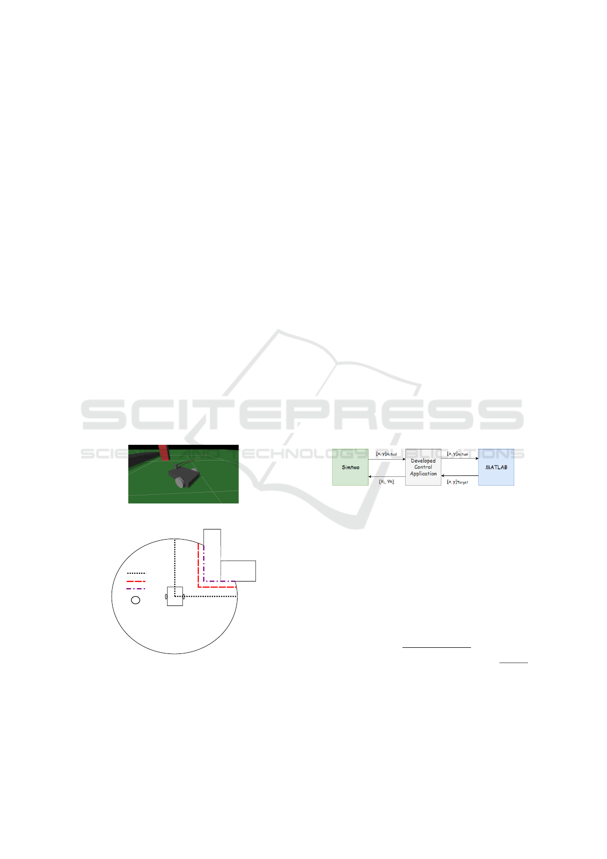
Figure 1: Robot Model SimTwo Environment.

Robot's Axes

Safe Distance

Laser Scan

LIDAR Range

Figure 2: LIDAR Structure Illustration.

In Figure 2, the purple dash-dotted line is what the

robot scans, i.e, the obstacles. The red dashed line,

for instance, is a safe threshold distance that the al-

gorithm applies to the detected obstacles to take into

consideration the size of the robot. In this way, it will

not collide when the algorithm generates a path. This

happens, because the algorithms will not consider this

new size as free space. In other words, for the avoid-

ance algorithms, the obstacle has its size increased by

a ∆d, which is the orthogonal distance between the

objects boundary and the red dashed line.

4 METHODOLOGY

The comparison approach will consider the longest

processing time (as the path planning is recalculated

every time a new obstacle is found), the execution

time, and ﬁnally, the distance travelled. The ﬁrst is

simply the longer processing time for the algorithm

to converge to the target point, which was, in this

case study, the ﬁrst time that the algorithm computed

the trajectory. The second, is the time that the robot

takes to reach the goal. The latter, will be the course

taken by the robot during the test. This distance will

be measured by odometry of the two wheel axes of

the differential geometry as explained in Section 3.2.

Note that the robot’s speed will be the same to all the

tests with both algorithms.

The processing time will be measured in MAT-

LAB where the algorithm codes run. For the execu-

tion time and distance traveled, both of them are mea-

sured in the simulator. Figure 3 illustrates the com-

munication between SimTwo and MATLAB.

Figure 3: System Structure.

The time starts to count when the robot moves and

only stops when it reaches the goal. The criteria to

check if the robot reaches the goal, is a Euclidean dis-

tance between the actual robot’s position and the goal

position. If the distance magnitude is less than 0.1,

then the code consider that the robot reached the goal.

In the same manner, the distance starts to be mea-

sured when the robot starts moving and stops when

the reaches the goal. The simulated encoder has 360

pulses per revolution in each axis. In this sense, the

distance traveled will be an arithmetic mean between

the two axes, Dist =

(Le ftAxis+RightAxis)

. In this sense,

the distance performed in each axis is, Axis =

(2×π×r)

360

which r is the wheel radius. Note that, Dist will be

measured in mm as the wheel radius will be expressed

in mm as shown in Section 3.

Several scenarios were tested for the algorithms.

In this work, two scenarios are presented. They

are similar, however with small adjustments that will

SIMULTECH 2019 - 9th International Conference on Simulation and Modeling Methodologies, Technologies and Applications

400

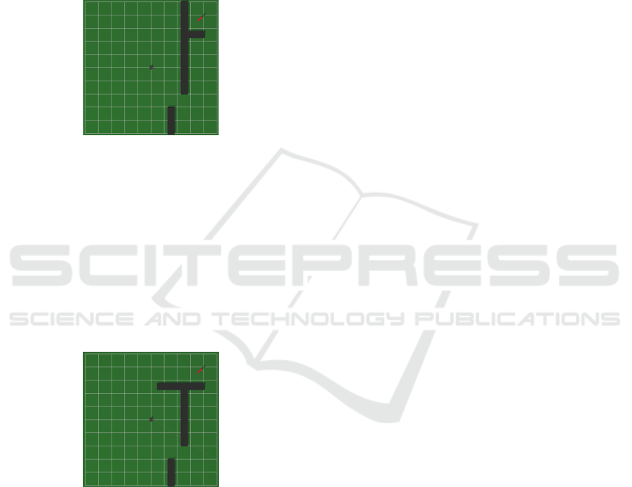
change both of the algorithm optimal paths. In the

ﬁrst scenario, the robot will start in the middle of the

map and its objective is to reach the red cuboid behind

the several obstacles in the northeast part of Figure 4.

It is clear that in Figure 4, the only possible path to the

other side of the walls in by the narrow gap between

the two walls in the southeast part of the Figure 4. It

is possible to assume that when the code starts to run,

the robot using a simulated LIDAR sensor described

in Section 3 sees only this gap.

Figure 4: First scenario test in SimTwo Environment.

In the second scenario, small adjustments were

made to force the algorithms to try out different ap-

proaches. As can be seen in Figure 5, when the sim-

ulation starts to run, the robot can not conclude that

the gap in the southeast part of the map is the only

possible path. In this way, it chooses the upper path

because it is shorter than the lower path. The robot

does not know if behind the upper walls in Figure 5

the path will be blocked. The explanation for each

algorithm for why it chooses the upper path will be

explained in their respective Sections 4.1 and 4.2.

Figure 5: Second scenario test in SimTwo environment.

As RRT* algorithm is a stochastic process, 10

tests were made for each scenario. This decision was

made not only because of the non-deterministic be-

haviour of the RRT* but also because in this way,

computing the mean and standard deviation, the com-

parison will be more reliable.

For A* algorithm in each scenario, the optimal

path will be the same in all tests. In this sense, the re-

sult ﬁgures of only one test will be presented for each

scenario. As for the non-deterministic behaviour of

RRT*, ﬁgures of two tests will be presented for the

ﬁrst and second scenarios.

4.1 A* Algorithm

The A* algorithm is one the most popular technique

used in path ﬁnding graph traversals. It takes best

of well-known Dijkstra’s and Best-First-Search algo-

rithms into account. For Dijkstra, it takes the part

that it favors the vertices closest to the starting point.

On the other hand, for Best-First-Search, it takes the

heuristics (favoring the cells that are closest to the

goal). The algorithm works by choosing a node ac-

cording to an f value, which is a cost value. This

value is a sum of the values g and h, f = g +h. In this

manner, at each step, it picks the node with the lowest

f , i.e, lowest cost.

The g value is the cost to move from the starting

point to another cell on the grid, according to the path

computed reach there. In the other hand, the h value

is an heuristic value, i.e, an estimated cost to move

from the node that you want to reach and the goal

destination node. This is called an ”educated guess”.

There are several ways to compute the h value and in

this work we used the euclidean distance.

The A* uses open and closed lists just like Dijk-

stra’s algorithm. The open set is a list of nodes that

are to be explored and the closed set is a list of nodes

already explored. In this way, as brieﬂy mentioned

above, at each step the node with the lowest f is re-

moved from the open set and the f and g values of its

neighbors are updated accordingly, and these neigh-

bors are added to the open set. The node removed

from the open set, is added to the closed set. The stop

criteria to the algorithm is when the open set is empty

or the goal node has an f value lower than any node

in the open set. After this, the cost of the goal node

is the lowest one. In this sense, to get the sequence

of movements from the starting point to the goal, A*

algorithm keeps track of the predecessor node called

parent node. So, the sequence is just listing every par-

ent node from the goal node until the start node. The

size of the A* cells considered are 1 m

. This choice

was made to match our simulation cells.

4.2 RRT* Algorithm

Rapidly Random Tree generates a tree by generating

random nodes in the free space. It starts from the start

node and expands until it reaches the target position

(node). At each iteration the tree expands by gener-

ating a new random node. If this node is not inside a

region that is considered an obstacle, then the nearest

node from the tree is searched. If this random node is

reached from the nearest node taking into considera-

tion the maximum step size, then the node is added to

the tree. Otherwise, it returns a new node by using a

A Comparison of A* and RRT* Algorithms with Dynamic and Real Time Constraint Scenarios for Mobile Robots

401

steering function, thus expanding the tree by connect-

ing the new node with the nearest node (Noreen et al.,

2016). Collision checks are performed every itera-

tion to ensure free connection between the new node

and the nearest node. RRT* for instance, works the

same way as RRT. However, it introduces two promis-

ing features called near neighbor search and rewiring

tree operations (Noreen et al., 2016). The ﬁrst feature

ﬁnds the best parent node for the new node consid-

ering a circle of radius r. It checks inside this circle

the parent node with the lowest cost before inserting

the three. It connects the lowest cost neighbor to the

new node. The latter feature, however, rewires the

tree inside of the same circle to maintain the tree with

minimal cost paths. In this work a maximum step size

of one meter per convenience is used.

5 RESULTS

Two scenarios were tested with ten tests each for each

algorithm. All conﬁgurations were also applied for

both, that is, all the physical characteristics of the en-

vironment and the sensors were applied in SimTwo

simulator to obtain the performance of A* and RRT*.

In this section, the results are presented and com-

pared.

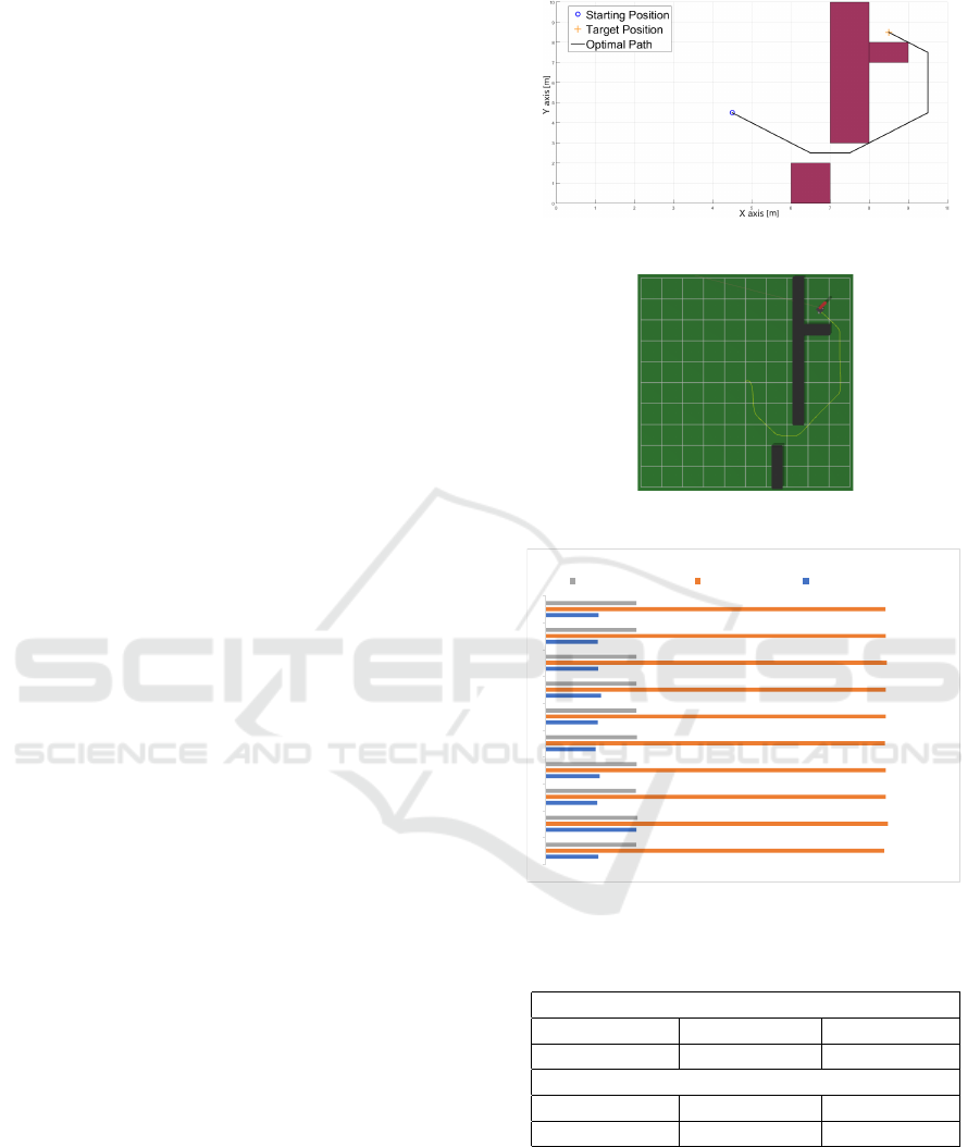
5.1 First Scenario

The ﬁrst scenario deals with the movement of the

robot starting from the center of the map, where the

end point is placed in the upper right corner, repre-

sented by the red cuboid. The A* algorithm is ex-

pected to calculate the trajectory, bypassing the ob-

stacles. Figure 6 illustrates the whole scenario with

the trajectory found.

As already mentioned, with the trajectory created,

the system sends the robot to reach the end point. Fig-

ure 7 shows the path traveled by the robot avoiding the

obstacles created in the SimTwo environment. The

entire analysis process in A* was repeated ten times

assuming that for each test, the system was restarted.

Then the data were collected and inserted in table for-

mat. Figure 8 reports the computation time, execution

time and distance traveled that the robot spent to per-

form the route with A* algorithm.

As can be noted, A* performs roughly the same

results in all ten tests, performing similar runs in each

test. The averages and standard deviations were com-

puted and Table 1 show all the data obtained in this

series of tests.

Figure 6: Illustration of path planned by A*.

Figure 7: Path performed by the robot in the ﬁrst scenario.

6.60

11.38

6.45

6.77

6.25

6.52

6.95

6.57

6.54

6.64

42.41

42.86

42.61

42.50

42.61

42.75

42.59

42.55

11.32

11.51

11.30

11.41

11.42

11.37

11.38

11.36

0.00 5.00 10.00 15.00 20.00 25.00 30.00 35.00 40.00 45.00 50.00

First scene in first test of A*

Distance traveled [m] Executing time [s] Processing time [ms/10]

Figure 8: Processing time, executing time and distance trav-

eled in ﬁrst scenario of A*.

Table 1: First Scenario A* Results.

Averages

Processing (s) Executing (s) Distance (m)

0.0706 42.6095 11.3805

Standard Deviations

Processing (s) Executing (s) Distance (m)

0.0144 0.1183 0.0554

As in the previous series of tests, they were ap-

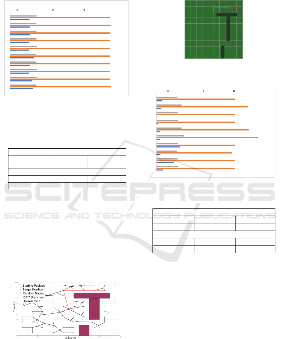
plied for RRT* algorithm. Figure 9 shows the tra-

jectory found to reach the target. After the trajectory

found by the RRT*, the developed system can already

send the information to the virtual robot. The environ-

ment of this approach can be seen in Figure 10.

All the analysis processed in RRT* was also re-

peated ten times considering that, for each test, the

SIMULTECH 2019 - 9th International Conference on Simulation and Modeling Methodologies, Technologies and Applications

402

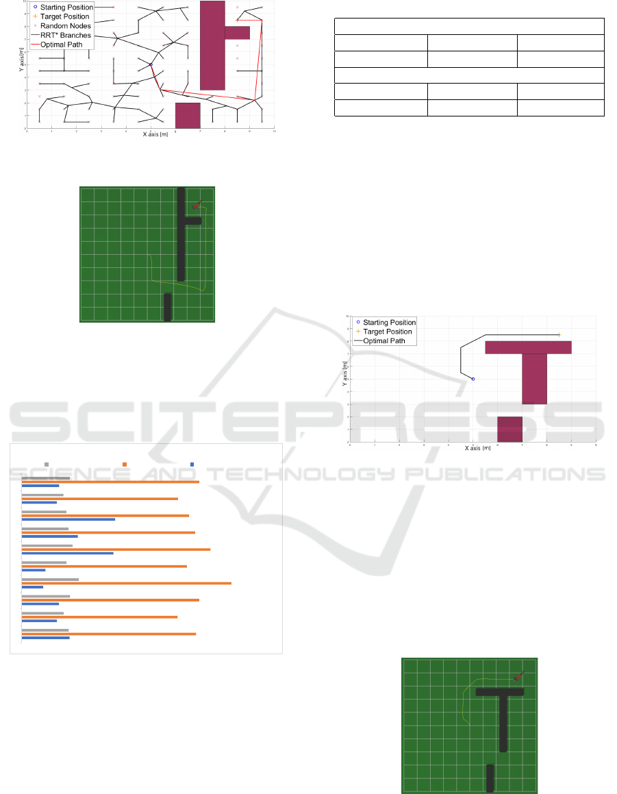
Figure 9: Illustration of path planned by RRT* in the ﬁrst

test.

Figure 10: Path performed by robot in the ﬁrst test.

system is also restarted. The data from the ten tests

are also in table format. Figure 11 shows the longest

computation time, executing time and distance trav-

eled that the robot took to perform the route with

RRT* algorithm.

13.47

9.95

10.51

6.13

6.73

25.66

15.73

26.13

9.86

10.54

48.67

43.53

49.55

58.53

46.11

52.72

48.39

46.74

43.66

49.63

13.23

11.80

13.59

15.97

12.57

14.27

13.18

12.56

11.74

13.50

0.00 10.00 20.00 30.00 40.00 50.00 60.00 70.00

First test in first scene of RRT*

Distance traveled [m] Executing time [s] Processing time [s]

Figure 11: Processing time, executing time and distance

traveled in ﬁrst scenario of RRT*.

Differently from A*, RRT* presents susceptible

differences in these tests, conﬁrming as mentioned

above. Computing the average and standard devia-

tion is possible to conclude that the path quality de-

pends heavily with more processing time, i.e, more

generated nodes. All these values are demonstrated in

Table 2.

Table 2: First Scenario RRT* Results.

Averages

Processing (s) Executing (s) Distance (m)

13.4712 48.7516 13.2409

Standard Deviations

Processing (s) Executing (s) Distance (m)

6.7515 4.2092 1.1815

5.2 Second Scenario

For the analysis of the second scenario, the initial

point of the robot is also the center of the map and

the target point is in the upper right corner. However,

in this analysis one of the obstacles has been opened

up. In this way, it is expected that the algorithms have

performances different from those obtained in the ﬁrst

scenario. Figure 12 shows the route found by A* for

this scenario and the movements of the virtual robot

in SimTwo, can be seen in Figure 13.

Figure 12: Illustration of path planned by A* in the second

scenario.

The paths generated by A* in Figure 12 and Fig-

ure 6 were different and this is expected due to the dif-

ference of the complexity of the scenarios. As in the

ﬁrst scenario, the tests were also repeated ten times

and for each time the system was also restarted. The

data of all of these tests are provided in table for-

mat. The processing time, execution time and dis-

tance traveled that the robot consumed to perform the

route with A* algorithm for this scenario is shown in

Figure 14.

Figure 13: Path performed by robot in the second scenario.

The averages and standard deviations are lower

than the ﬁrst scenario and this is expected since this

A Comparison of A* and RRT* Algorithms with Dynamic and Real Time Constraint Scenarios for Mobile Robots

403

6.13

5.90

5.03

5.29

6.28

5.04

5.16

5.39

5.27

5.20

26.48

26.34

26.28

26.34

26.22

26.28

26.33

26.31

26.44

26.33

7.00

7.10

7.13

6.97

7.00

7.12

7.02

6.99

6.98

7.03

0.00 5.00 10.00 15.00 20.00 25.00 30.00

First scene in second test of A*

Distance traveled [m] Executing time [s] Processing time [ms/10]

Figure 14: Processing time, executing time and distance

traveled in second scenario of A*.

scenario is less complex. The data are displayed in

Table 3.

Table 3: Second Scenario A* Results.

Averages

Processing (s) Executing (s) Distance (m)

0.0546 26.3355 7.0354

Standard Deviations

Processing (s) Executing (s) Distance (m)

0.0043 0.0724 0.0585

In this second scenario, the same test is also car-

ried out for RRT* performance analysis. Figure 15

indicates the route calculated by the RRT * algorithm.

The virtual robot movement in the simulated environ-

ment SimTwo is shown in Figure 16.

All the paths are similar as the distance to reach

the goal is considerably lower than scenario one and,

because of that, the algorithm converge much more

faster, generating similar paths. The results are pre-

sented below. Figure 17 shows the processing time,

execution time and distance traveled of the robot by

performance with RRT*.

Figure 15: Illustration of path planned by RRT* in the sec-

ond scenario during test one.

The averages and standard deviations are mea-

sured and Table 4 reports them. Again, the values are

lower due to the complexity of the scenario.

Figure 16: Path performed by robot in the second scenario

during test one.

2.30

6.19

1.39

8.31

1.31

1.19

0.62

0.22

1.70

1.93

27.48

27.45

26.50

27.41

35.55

32.38

27.45

27.44

32.02

27.44

7.50

7.37

7.20

7.38

9.65

8.78

7.50

8.74

7.38

0.00 5.00 10.00 15.00 20.00 25.00 30.00 35.00 40.00

Second test in second scene of RRT*

Distance traveled [m] Executing time [s] Processing time [s]

Figure 17: Processing time, executing time and distance

traveled in second scenario of RRT*.

Table 4: Second Scenario RRT* Results.

Averages

Processing (s) Executing (s) Distance (m)

2.5156 29.111 7.8997

Standard Deviations

Processing (s) Executing (s) Distance (m)

2.4799 2.8979 0.7949

6 CONCLUSION AND FUTURE

WORK

This paper addressed the comparison of performance

for two path planning algorithms considering the

physical inﬂuences of the environment with a mobile

robot. For the ﬁrst scenario, RRT* performed worse

in all tests. Processing roughly 190 times slower

than A*. As for execution time, both performed sim-

ilar, RRT* a slightly slower, 14.41%. In relation

to the distance traveled, both performed similarly as

well. RRT* generating a slightly longer path than A*,

16.34%.

For the second scenario, RRT* performed worse

in all tests. Regarding processing time, it performed

45 times slower than A*. For execution time, RRT*

SIMULTECH 2019 - 9th International Conference on Simulation and Modeling Methodologies, Technologies and Applications

404

performed 10.54% slower than A*. Finally for dis-

tance traveled, RRT* performed 12.28% slower than

A*. For both scenarios regarding the standard devia-

tion, it is concluded that, as the complexity of the en-

vironment increases the standard deviation increases

for both algorithms. However, as RRT* has non-

deterministic behaviour, it increases by a higher order

of magnitude than A*. In addition, if the cell size for

A* was reduced, i.e, the map resolution increases, the

memory and processing time required would increase

exponentially.

For future work tests with both algorithms will be

implemented in a real scenario.

ACKNOWLEDGEMENTS

This work is ﬁnanced by the ERDF – European

Regional Development Fund through the Opera-

tional Programme for Competitiveness and Interna-

tionalisation - COMPETE 2020 Programme within

project POCI-01-0145-FEDER-006961, and by Na-

tional Funds through the FCT – Fundac¸

ao para

a Ci

encia e a Tecnologia (Portuguese Foundation

for Science and Technology) as part of project

UID/EEA/50014/2013.

REFERENCES

Bohlin, R. and Kavraki, L. E. (2000). Path planning us-

ing lazy prm. In Proc. ICRA. Millennium Conf. IEEE

Inter. Conf. on Robotics and Automation. Symposia

Proc., volume 1, pages 521–528. IEEE.

Brito, T., Lima, J., Costa, P., and Piardi, L. (2017). Dy-

namic collision avoidance system for a manipulator

based on rgb-d data. In Iberian Robotics conference,

pages 643–654. Springer.

Cheng, Y. and Wang, G. Y. (2018). Mobile robot navigation

based on lidar. In 2018 Chinese Control And Decision

Conference (CCDC), pages 1243–1246. IEEE.

Choset, H. M., Hutchinson, S., Lynch, K. M., Kantor, G.,

Burgard, W., Kavraki, L. E., and Thrun, S. (2005).

Principles of robot motion: theory, algorithms, and

implementation. MIT press.

Ducho

n, F., Babinec, A., Kajan, M., Be

no, P., Florek, M.,

Fico, T., and Juri

sica, L. (2014). Path planning with

modiﬁed a star algorithm for a mobile robot. Procedia

Engineering, 96:59–69.

He, D.-Q., Wang, H.-B., and Li, P.-F. (2018). Robot

path planning using improved rapidly-exploring ran-

dom tree algorithm. In 2018 IEEE Industrial Cyber-

Physical Systems (ICPS), pages 181–186. IEEE.

Kavraki, L., Svestka, P., and Overmars, M. H. (1994).

Probabilistic roadmaps for path planning in high-

dimensional conﬁguration spaces, volume 1994. Un-

known Publisher.

Lima, J. and Costa, P. (2017). Ultra-wideband time of ﬂight

based localization system and odometry fusion for a

scanning 3 dof magnetic ﬁeld autonomous robot. In

Iberian Robotics conf., pages 879–890. Springer.

Lima, J., Gonc¸alves, J., and Costa, P. J. (2015). Modeling of

a low cost laser scanner sensor. In CONTROLO’2014–

Proceedings of the 11th Portuguese Conference on

Automatic Control, pages 697–705. Springer.

Loong, W. Y., Long, L. Z., and Hun, L. C. (2011). A star

path following mobile robot. In 2011 4th Inter. conf.

on mechatronics (ICOM), pages 1–7. IEEE.

Moon, C.-b. and Chung, W. (2015). Kinodynamic planner

dual-tree rrt (dt-rrt) for two-wheeled mobile robots us-

ing the rapidly exploring random tree. IEEE Trans. on

indust. electro., 62:1080–1090.

Noreen, I., Khan, A., and Habib, Z. (2016). A comparison

of rrt, rrt* and rrt*-smart path planning algorithms.

Inter. Jrnl. of Comp. Sci. and Net. Sec., 16(10):20.

Okubo, Y., Ye, C., and Borenstein, J. (2009). Characteriza-

tion of the hokuyo urg-04lx laser rangeﬁnder for mo-

bile robot obstacle negotiation. In Unmanned Systems

Technology XI, volume 7332, page 733212. Inter. Soc.

for Opt. and Phot.

Piardi, L., Lima, J., and Costa, P. (2018). Development of

a ground truth localization system for wheeled mobile

robots in indoor environments based on laser range-

ﬁnder for low-cost systems. In Proc. of 15th In-

ter. Conf. on Informatics in Control, Automation and

Robotics-ICINCO’18, pages 341–348. SciTePress.

Plaku, E., Bekris, K. E., Chen, B. Y., Ladd, A. M., and

Kavraki, L. E. (2005). Sampling-based roadmap of

trees for parallel motion planning. IEEE Transactions

on Robotics, 21(4):597–608.

Schwartz, J. T. and Sharir, M. (1983). On the “piano

movers” problem. ii. general techniques for comput-

ing topological properties of real algebraic manifolds.

Adv. in applied Mathematics, 4:298–351.

Ye, C. and Borenstein, J. (2002). Characterization of a 2d

laser scanner for mobile robot obstacle negotiation. In

Proc. IEEE Inter. Conf. on Robotics and Automation,

volume 3, pages 2512–2518. IEEE.

A Comparison of A* and RRT* Algorithms with Dynamic and Real Time Constraint Scenarios for Mobile Robots

405