A Method for Health Detection in Eureka Based on Load Forecasting

Chao Deng

, Xinming Tan

and Lang Li

School of Computer Science &Technology, Wuhan University of Technology

Wuhan, Hubei

Keywords: Microservice, Health detection, Time series, Load forecasting.

Abstract: Health detection relies on the heartbeat mechanism in Eureka. The heartbeat mechanism analyzes the status

of service by periodically detecting the running status of the service node. But it doesn't care whether the

service runs successfully, therefore reducing the success rate of service calls. In order to solve the problem,

this paper proposes a new method for load forecasting based on time series. The value of load forecasting is

used to measure the health of the service node quantitatively, and the number of available instances is

effectively reduced during load balancing and the load balancing efficiency was improved.

1 INTRODUCTION

With the rapid development of computer network, the

drawbacks of the traditional application architecture

become more and more obvious, which seriously

restrict the rapid innovation and agile delivery of the

business (Zheng Mingzhao et al. 2017). The

microservice architecture was proposed to solve the

problems in traditional application architectures

(Lewis et al. 2014).

Spring Cloud is an open source microservice

development tool based on Spring Boot. Spring

Cloud Eureka module has been used for service

governance, and providing services such as health

detection. At present, the health detection in Spring

Cloud Eureka relies on the heartbeat mechanism

(Smaoui et al. 2017). The mechanism gets the running

status of service by periodically detecting the running

status of the service node, regardless of whether the

service can run successfully. This approach will have

resulted in some failed service calls, which will

reduce the success rate of service calls. In order to

solve the above problem, a health detection method

based on load forecasting for quantitative analysis of

service health has been proposed. In this method,

while monitoring the performance indicators, the

health of the service node is measured quantitatively

by the load forecasting value.

Load balancing technology is the focus of

research in distributed architecture. The research

direction mainly focuses on the load balancing

algorithm, which is divided into static load balancing

algorithm and dynamic load balancing algorithm.

Static load balancing algorithm does not consider the

actual load status of the server generally. Although

the implementation of static load balancing algorithm

is simple, the effect is not good mostly. Dynamic load

balancing algorithm requires that service load

information can be sent in smaller time intervals, even

in real time, which results in significant consumption

of server resources. Therefore, some people proposed

some load forecasting algorithms. Li Qinghua and

Guo Zhixin (2002) proposed a BP forecasting

algorithm based on artificial neural network. Xu

Jianfeng f et al. (2000) proposed a forecasting

algorithm based on filtering theory. Meng Limin and

Xu Yang (2016) proposed a load forecasting

algorithm based on dynamic index. Wolski et al.

(2000) proposed a forecasting algorithm based on

CPU utilization in UNIX system. Yuan Gang (2015)

proposed a load forecasting algorithm based on

service classification. Yang Wei et al. (2006)

proposed a load forecasting algorithm based on time

series and so on.

The algorithms proposed in [4-6] are relatively

complicated. The algorithms did not consider the

resource consumption of the load forecasting, which

will have affected the execution efficiency of the

service node. The algorithms proposed in [7-8]

calculated the current load value of the service

quantitatively, and calculated the load forecasting

value comprehensively by monitoring the number of

service requests, without considering the relationship

between the load values at different time (Dinda

Deng, C., Tan, X. and Li, L.

A Method for Health Detection in Eureka Based on Load Forecasting.

DOI: 10.5220/0008098902270232

In Proceedings of the International Conference on Advances in Computer Technology, Information Science and Communications (CTISC 2019), pages 227-232

ISBN: 978-989-758-357-5

227

1998). Therefore the accuracy of the prediction could

not be guaranteed. The algorithm proposed by Yang

Wei et al. (2006) was based on the time series of the

load, but it did not provide a detailed measure of the

load value. Based on the above considerations, this

paper proposes a load forecasting method based on

the time series of the load, and considers the

dependence of different service nodes on host

resources, and gives a quantitative measure of load

value.

In summary, this paper proposes an improvement

measure for Eureka's health detection. It provides

more data support for system load balancing by

distinguishing between normal service and fault

service by running monitoring and load forecasting of

service node.

2 LOAD FORECASTING MODEL

2.1 The Calculation of Load

The load is a reflection of the current performance of

the server. In order to make full use of the resources

of all service nodes and improve resource utilization

and system execution efficiency, the performance

status of the server must be accurately measured.

Indicators such as CPU utilization, memory

utilization, disk I/O utilization, network bandwidth

utilization, and the count of server processes usually

affect the load on the server. Yang Mingji et al. (2016)

proposed a load calculation method based on CPU

utilization and memory utilization. The calculation of

the load in the method was not sufficient for the

utilization of performance indicators. This paper

proposes a load calculation method that

comprehensively considers CPU utilization, memory

utilization, disk I/O utilization, and network

bandwidth utilization.

The load on the server is highly correlated with its

own hardware utilization. These factors have

different effects on server performance. The

following two aspects should be noted when selecting

hardware load indicators:

(1) The indicator should be collected

conveniently, and the collection process is basically

non-intrusive to the load balancing process.

(2) Appropriate indicator is selected under

conditions of high accuracy and low computational

overhead.

The load of a service node usually includes two

aspects: hardware resource utilization and the number

of the service consumer. Hardware resources

determine the ability of a service node to process

service requests. The more threads in the service node,

the more resources are consumed. Therefore, the

change in hardware resource utilization can

intuitively reflect the actual load of the service node.

In summary, this paper selects CPU utilization,

memory utilization, I/O occupancy rate and network

bandwidth utilization to calculate the comprehensive

load of the server. These indicators can reflect the

actual load of the service load.

The calculation formula is shown in Equation 1.

100*)

4321

NkIkMkCkX （

(1)

Where X is the integrated load, C is the CPU

utilization, M is the memory utilization, I is the I/O

utilization, N is the network bandwidth utilization, k

is a coefficient, and the magnitude of k

represents the

degree of importance of the four indicators, and their

values satisfy the Equation 2.

1 2 3 4

+ + + =1k k k k

(2)

Different service nodes provide different services,

so the service nodes have different degrees of

dependence on various indicators. We assign

different values to different service nodes

dynamically.

2.2 Time Series Model

It can be seen from the characteristics of the load that

the load is a time series, and the load value shows a

strong correlation with time, so this paper proposes a

load forecasting algorithm based on the time series

model.

The theory of time series summarizes a number of

time series models describing stochastic processes.

Common models are AutoRegressive model (AR

model), Moving Average model (MA model), and

AutoRegressive Moving Average models (ARMA

model).

Generally, which model should be selected for

fitting needs to be distinguished according to the

tailing or truncation characteristics of the

autocorrelation coefficient and partial autocorrelation

coefficient of the time series.

If the autocorrelation coefficient is tailing and the

partial autocorrelation coefficient is truncation, the

AR model is suitable. If the autocorrelation

coefficient is truncation and the partial

autocorrelation coefficient is tailing, the MA model is

suitable. If the autocorrelation coefficient and the

partial autocorrelation coefficient are tailing, the

ARMA model is suitable.

Through the collection of multiple sets of data,

this paper finds that the time series of load obtained

through calculations all fluctuate randomly within a

certain range, and the series presents a certain degree

CTISC 2019 - International Conference on Advances in Computer Technology, Information Science and Communications

228

of stability. And the autocorrelation coefficient is

tailing, the partial autocorrelation coefficient is

truncation in most series. Therefore, the AR model is

used in this paper.

The AR model describes a simple autoregressive

stochastic process whose mathematical

representation is shown in Equation 3.

=a +a +a + +a

t 0 1 t-1 2 t-2 p t p t

x x x x





 

(3)

Where a

is a parameter,

{}



is white noise. The

time series value

can be expressed by the sequence

value of the previous p moments and the current noise.

The p order autoregressive model, abbreviated as

AR(p) model, is an AR model that predicts the next

sequence value based on the sequence values of the

previous p moments.

a = (a ,a , ,a )

0 1 p



is the

autoregressive coefficient in the AR(p) model, and

{}



obeys the distribution

(0, )N



For a time series

{}

, the modelling process of

the AR model is shown in Figure 1.

Figure 1: The modelling process of AR model.

2.3 Test for Stationary

If the mean of a time series is constant and the

variance does not exhibit a time-varying

characteristic, then it can be called a stationary

sequence. The autocorrelation coefficient and partial

autocorrelation coefficient of the stationary sequence

exhibit tailing or truncation characteristics. Therefore,

the stationarity test can be performed by the

autocorrelation coefficient and the partial

autocorrelation coefficient of the sequence. The

mathematical representation of the P-order

autocorrelation coefficient is shown in Equation 4.

( )( )

i i p

x u x u

















(4)

Where u has the meaning shown in Equation 5,

and



has the meaning shown in Equation 6.

If the autocorrelation coefficient and partial

autocorrelation coefficient of sequence exhibit tailing

or truncation characteristics as the order increases,

then the sequence is a stationary sequence.

2.4 Parameter Estimation

The parameter estimation in the AR model is usually

the least square estimation.

For the load sequence

{}

, if its mean is not zero,

the sequence should be converted to a zero-sequence

{ | }

t t t

w w x u

For a time series

{}

, when

1ip

, the

estimation of



is represented by



which has the

meaning shown in Equation 7.

ˆ ˆ ˆ ˆ

-(a +a + +a )

i i 1 i-1 2 i-2 p i p

w w w w





 

(7)

Where



is residual. The goal of parameter

estimation is to minimize the sum of squared

residuals. We define a in Equation 8, define W in

Equation 9, and define Y in Equation 10.











(8)

n n n p

w w w





  







(9)









(10)

Then the sum of squared residuals can be

expressed as Equation 11.

(a) ( a) ( a)

F Y W Y W  

(11)

In the Equation 11, we obtain the derivation of

parameter a and then let the derivation equals 0. The

parameter a in Equation 12 is obtained. The parameter

estimation of the model was obtained.

a ( )

W W W Y





(12)

2.5 Tests for Forecasting Model

After the model is fitted, it is necessary to test the

validity of the model to determine whether the fitting

model is sufficient to extract the information in the

sequence. A good fit model should be able to extract

almost all of the sample-related information in the





(5)

= ( )









(6)

Model

identification

Model

identification

Parameter

estimator

Parameter

estimator

Sequence

Smoothing

Sequence

prediction

Sequence

prediction

End

White noise

test

White noise

test

Model

checking

Model

checking

Stationarity

test

Stationarity

test

A Method for Health Detection in Eureka Based on Load Forecasting

229

sequence values. This paper proposes a method to test

the validity of the fitted model.

{}



is white noise, the autocorrelation

coefficients of all its orders are theoretically zero.

Considering the deviation of the data, most

autocorrelation coefficients should be in the vicinity

of zero. This means that the model takes into account

relevant information for almost all samples.

Therefore, the validity of the model can be confirmed

by a white noise test of the

{}



3 IMPLEMENT

Health detection is part of service governance in

Eureka. Service governance in Eureka includes three

core elements: service registry, service provider, and

service consumer. The entire calling process of the

service is shown in Figure 2.

Service provider 1

Service provider N

Instances list

Service consumer

Is the heartbeat

signal times out?

Is the heartbeat

signal times out?

Eureka Server

Service eviction

Service renew

service call

obtain

instances

obtain

instances

heartbeat

signal

heartbeat

signal

heartbeat

signal

heartbeat

signal

Figure 2: The calling process of service in Eureka.

In Eureka, the registration center does not care

about the status of the service, but only records the

status of the service. In the heartbeat mechanism, as

long as the program is running, it is judged that the

service is healthy and available by default, which is

obviously not accurate enough. This paper proposes

an improved scheme based on the load forecasting

model. The entire calling process of the service is

shown in Figure 3.

Service

provider 1

Service

provider 1

Service

provider N

Service

provider N

Instances list

Service consumer

Eureka Server

service call

obtain

instances

obtain

instances

Monitoring

component

Monitoring

component

Actuator

monitoring

load

monitoring

load

service

renew

service

renew

Is the heartbeat

signal times out?

Is the heartbeat

signal times out?

service eviction

service renew

Figure 3: The improved calling process of service in the

Eureka.

The load forecasting model works in the

monitoring component, and the workflow is as the

following:

 The service provider registers the service

instance in the service registry;

 The service provider starts the spring-boot-

actuator module and uses the Sigar monitoring

component to periodically obtain service

performance indicators;

 Calculate the load value by the load value

calculation method, and save it in the Map;

 Input the load sequence in the Map to the load

forecasting model, a load forecasting value of

the service instance will be outputted;

 The service registry accesses the /health

endpoint of the spring-boot-actuator module

periodically;

 The /health endpoint obtains the load

forecasting value of the service instance, and

returns the service running status according to

the monitoring result of the service, and

updates the load value of the service instance in

the registration center;

 The service consumer obtains a list of service

instances, and completes instance selection and

invocation according to the load forecasting

value combined with the load balancing policy.

4 EXPERIMENTAL RESULTS

In order to verify the validity and feasibility of the

forecasting model, we carry out the following

experiments.

The parameter p of the time series model is larger,

the prediction cost is higher. In order to reduce the

complexity of the experimental evaluation, we choose

5, 10, 15 as the candidate parameters. The time

interval of the sequence value will have a certain

impact on the forecasting model. We choose 1s, 5s,

10s, 20s as the candidate parameters, and use the two

indicators in Equation 13 and Equation 14 to predict

and evaluate different parameters.

= ( )

err err









(13)

err







(14)

The meanings of

err

and

err

are shown in

Equation 15 and Equation 16.

t t t

err x x

(15)

CTISC 2019 - International Conference on Advances in Computer Technology, Information Science and Communications

230

err err





(16)

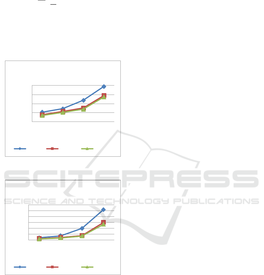
The average ratio λ and the variance δ

of the

prediction errors are used as indicators for evaluating

the forecasting model. The smaller the variance is, the

more stable and accurate the forecasting is. The

experimental results are shown in Figure 4 and Figure

Figure 4: Comparison of the average ratio of prediction

errors.

Figure 5: Comparison of the variance of prediction

errors.

According to the above experimental results, as

the time interval increases, the average ratio and the

variance of the prediction error in model of each order

show an upward trend, which means the shorter the

time interval for monitoring the load value, the

smaller the error of the load forecasting value and the

smaller the error range. With the increase of the order,

the average ratio and the variance of the prediction

errors in model of each time interval show a

downward trend, which means the more load values

referenced in the model, the smaller the error of the

load forecasting value and the smaller the error range.

The 5th order model has fewer prediction

reference values, so the accuracy of the predicted

value changes relatively with the change of the time

interval. The evaluation index difference between the

10th order model and the 15th order model is small.

In order to reduce the complexity of the model, the

10th order model is selected. For the 10th order model,

when the time interval is less than 10 seconds, the

average of the prediction error is less than 8%, the

variance of the prediction error is less than 4. When

the time interval is 20 seconds, the average of the

prediction error is close to 15%. Since time is

required between transmitting the load forecasting

value and using the load forecasting value, the time

interval of 10 seconds is selected for modeling.

5 CONCLUSIONS

The current service health detection heartbeat

mechanism in Eureka can only detect whether the

service is online. And through the Spring-boot-

actuator module, the operating status can be

monitored before and after service registration. Based

on this, this paper adds the load information

monitoring component to monitor the load

information of the service node by means of the

Spring-boot-actuator module. Then the load

forecasting model is used to predict the load value

after a period of time and the load value will be fed

back to the registry. This method adds very little

overhead to the service provider, but the service

consumer can accurately obtain the load status of

each instance providing the same service from the

experimental results. Combined with the load

balancing algorithm, the consumer can call the

appropriate service instance more reasonably. Finally,

how the load balancing component in Ribbon client

combines the existed load balancing strategy with

load forecasting values in the service consumer will

be the direction of future research.

REFERENCES

Zheng M J, Zhang J Q. (2017), Discussion on the Evolution

of Big Platform System Architecture Based on

Microservice. Computer Engineering & Software,

38(12), p165-169.

0.05

0.1

0.15

0.2

1 5 10 20

Average error ratio

Time interval/second

Comparison of the average ratio of

prediction errors

5th order 10th order 15th order

1 5 10 20

variance

Time interval/second

Comparison of the variance of

prediction errors

5th order 10th order 15th order

A Method for Health Detection in Eureka Based on Load Forecasting

231

LEWIS J, FOWLER M. (2014), Microservices [online]. A

vailable at: http://martinfowler.com/articles/microservi

ces.html [Accessed 20 February 2019].

Smaoui G, Abid M. (2017), Development and

benchmarking of algorithm for heartbeat detection.

2017 International Conference on Smart, Monitored

and Controlled Cities (SM2C), p87-90.

Li Q H, Guo Z X. (2002), Approach to load prediction of

networks in workstations. Journal of Huazhong

University of Science and Technology(Natural Science

Edition), 30(06), p49-51.

Xu J F, Zhu Q B and Hu N. (2000), Predictive scheduling

algorithm in distributed real-time systems. Journal of

Software, 11(01), p95-103.

Meng L M, Xu Y. (2016), Load balancing algorithm based

on dynamic exponential smoothing prediction. Journal

of Zhejiang University of Technology, 44(04), p379-

382.

Wolski R , Spring N T and Hayes J. (2000), Predicting the

CPU Availability of Time-shared Unix Systems on the

Computational Grid. Cluster Computing, 03(04), p293-

301.

Yuan G. (2015), A Dynamic Load Balancing Scheduling

Algorithm Based on Service Differentiation and

Prediction. Computer Technology and Development,

25(06), p96-100.

Yang W, Zhu Q M and Li P F. (2006), Server Load

Prediction Based on Time Series. Computer

Engineering, 32(19), p143-145.

Dinda P. (1998), The statistical properties of host load.

Proceedings of the Fourth Workshop on Languages,

Compilers, and Run-time Systems for Scalable

Computers, p211-229.

Yang M J, Wang H and Zhao J F. (2016), Research on

Load Balance Algorithm Based on the Utilization Rate

of the CPU and Memory. Bulletin of Science and

Technology, 32(04), p160-164.

CTISC 2019 - International Conference on Advances in Computer Technology, Information Science and Communications

232