
Sphere Localization from a Minimal Number of Points in a Single
Image
Kunfeng Shi
1
, Xuebin Li
1
, Huikun Xu
1
, Hongmei Zhao
1
and Huanlong Zhang
1
1
School of Electrical and Information Engineering, Zhengzhou University of Light Industry, Zhengzhou, China
Keywords: Sphere localization, Three-point algorithm, Ellipse fitting, Grbner basis
Abstract: This paper proposes a new three-point method to locate the spatial sphere center from a single image. In
monocular vision system with known intrinsic parameters, the traditional methods of locating the center of a
spatial sphere with known radius require fitting its image points to an ellipse from which the sphere center is
extracted. The ellipse fitting procedure requires at least five image points whereas the projection ellipse of a
sphere essentially is a three-degree-of-freedom problem, which implies that over-parametrization is
introduced in ellipse fitting. In this paper, the ellipse is represented with the three coordinates of the sphere
center, and then at least three image points on the ellipse are used to construct a set of quadratic equations of
the coordinates from which the Grbner basis method is used to solve for the coordinates. The experimental
results show that the three-point method can solve the problem with less than five image points, and when
the number of image points increases to five or more, the new method can also improve sphere localization
accuracy and have improved robustness.
1 INTRODUCTION
Due to the characteristic of rotation symmetry of the
sphere in space, it not only has a good image contour
continuity, but also has less requirements to camera
shooting angles and shielding problems (Zhao et al.,
2014; Liu et al., 2016). Therefore, it has attracted
extensive attention and research in camera
calibration and target localization, especially in
multi-camera calibration (Gu et al., 2012; Shi et al.,
2012; Shi et al., 2014). In recent years, camera
localization technology based on spherical targets
has been applied to robotic astronauts (Fan et al.,
2016) and laser tracking visual guidance (Wei et al.,
2012). In addition, due to the advantages of
portability and easy operation (Zheng et al., 2018),
the localization of handheld spherical targets has a
good application prospect in video capture systems.
At present, in the research on the positioning of
spherical targets, (Zhao et al., 2014) proposed a
method to calculate the projection point of the
sphere center by using the axis of symmetry and
common tangent of two projection conics. However,
this method is applicable to the condition that an
image containing two spheres at different positions
in space must be taken, and the resulting image must
also be an ellipse. (Fan et al., 2016; Wei et al., 2012;
Shui and Ahmad, 1989; Wong et al., 2008) first
deduced a right circular cone tangent to a space
sphere based on the image ellipse of the sphere, and
then calculated the center of the sphere based on the
right circular cone equation and its geometric
characteristics. This method depends on the fitting
of the sphere image ellipse, and the accuracy of
fitting also determines the positioning accuracy of
the sphere center. (Liu et al., 2016; Gu et al., 2012;
Sun et al., 2016) established a spherical pinhole
imaging model, derived a geometric relationship
between the elliptic center and the imaging point of
the sphere center, and then obtained a more accurate
coordinates of the projection point of the sphere
center through distortion correction. This method is
not only complicated in theoretical derivation, but
also needs to fit an ellipse. Among them, the method
proposed in (Gu et al., 2012) also requires that the
compensation coefficient must be calculated by at
least six spatial spheres before compensation, and
this method will fail when the ratio of the radius of
the sphere and the distance from the sphere center to
the optical center exceeds a certain range. Recently,
(Geng et al., 2018) proposed a new method of
distortion correction for the coordinates of imaging
edge points, and extracting the coordinates of
Shi, K., Li, X., Xu, H., Zhao, H. and Zhang, H.
Sphere Localization from a Minimal Number of Points in a Single Image.
DOI: 10.5220/0008096300650070
In Proceedings of the International Conference on Advances in Computer Technology, Information Science and Communications (CTISC 2019), pages 65-70
ISBN: 978-989-758-357-5
Copyright
c
2019 by SCITEPRESS – Science and Technology Publications, Lda. All rights reserved
65

spherical center projection point in conjunction with
the focal length. From the above analysis, it is not
difficult to see that, except for the method in (Geng
et al., 2018), existing methods need to fit the image
edge points. Since the fitting of an ellipse requires at
least five measuring points, when the number of
measuring points extracted from the ellipse image is
less than five, the traditional methods mentioned
above will not be able to locate the sphere, which
undoubtedly makes the traditional methods have
some limitations.
The contribution of this paper is that the conic of
the projection ellipse of the sphere in a camera is
represented by the three-dimensional coordinates of
the sphere center, and then the sphere center is
extracted by minimizing the distance from the image
point to the ellipse. The new method enables the
single-view sphere center positioning based on at
least three image points and avoids over-
parametrization in traditional methods. The new
method has higher sphere localization accuracy and
robustness with five or more image points.
2 THREE-POINT METHOD
2.1 Theoretical Analysis of Three-Point
Method
Without loss of generality, let’s denote the camera
calibration matrix is , the three-dimensional
coordinates of the spherical center in the camera
coordinate system is
, the conic of the
spherical imaging ellipse is , the sphere radius is
and the measuring points are
,
. Matrix
is an n-order identity matrix. In
addition, the image is normalized by
to
eliminate the influence of .
The conic of the projection ellipse of the sphere
in the camera is represented by the three-
dimensional coordinates of the sphere center as
. (1)
Then, the sphere center can be extracted by
minimizing
, (2)
It’s subject to the constraint in equation (1). This
minimization problem can be solved in the manner
similar to the method in (Stewénius et al., 2006).
Firstly, from the following set of equations
, (3)
we can get
. (4)
After substituting coordinates, the equation (4) can
be expressed as
. (5)
When the number of measurement points , by
stacking such equations as (5), we have
. (6)
Let be the coefficient matrix of equations (6),
is the unknown vector
of equations (6). In addition, if we label the vector
, then this
set of equations (6) can be rewritten as
. (7)
Let
be the rank three approximation of
computed with the first three principal components.
The solution of the system is composed of a
particular solution and a free solution in the null
space. The particular solution is
. (8)
Here,
is the pseudo inverse of
.The free
solution can be represented with the three singular
vectors
of the matrix corresponding
the smallest three singular values. Then,
. (9)
Here (
) are three unknowns to be
computed later. For the convenience of the
following, let us denote
CTISC 2019 - International Conference on Advances in Computer Technology, Information Science and Communications
66

T
. Recall the definition
and therefore the six
elements of obey the following internal
constraints.
. (10)
Equations (10) are actually six quadratic
equations on the unknowns
. Define the
monomials vector
(11)
Equations (10) can be rewritten as
, (12)
Here is a 6×10 matrix. After Gauss-Jordan’s
elimination, equation (12) can be rewritten as
. (13)
Here
is a 6×6 identity matrix and is a 6×4
matrix. Let
. Now, we define the
basis monomials vector
T
. (14)
Let
be any
in
, then construct
the action matrix
with equation (12) that obeys
. (15)
Here, the elements in
can be expressed with
the elements in according to the choice of
.
Denote the i-th row of as
, and then when
,
, and
respectively, the three versions of
are computed as
. (16)
Four complex solutions of
are computed as
the eigenvectors of
. For stability reasons, three
matrices
are computed for
being
,
and
respectively, and then the matrix
with the
largest norm is used to compute . Then, the
value of the unknown parameter vector can be
extracted from . Note that the last element of
the eigenvectors of the
matrix should be
normalized to 1.
Then, the real solutions of are back-substitute
into equation (9), and at most four real solutions of
can be obtained. It is particularly noteworthy that
since the depth of the sphere center is real and
positive, the solutions with negative
should be
excluded. After the exclusion, the three-dimensional
coordinates of the sphere centre are extracted from
the solutions of as follows
. (17)
The three-dimensional coordinates of the sphere
center have at most four real solutions, but after
enforcing the condition that, generally only
one solution is obtained.
2.2 Maximum Likelihood Estimation
The solution of the sphere center coordinates
obtained by the above method can be optimized
through maximum likelihood method. An image
point on the projection ellipse of the sphere can be
represented by
,
and , where
is
the angle parameter of the image point on an ellipse.
Therefore, the image point on the ellipse can be
represented as in equation (18) at the bottom of this
page.
Assume that the measurement points are
corrupted by Gaussian white noise. The maximum
likelihood estimate can be obtained by minimizing
the following functional:
. (19)
Minimizing (19) is a nonlinear minimization
problem, which is solved with the sparse Levenberg-
Marquardt algorithm as described in (Hartley and
Zisserman, 2004).
(18)
Sphere Localization from a Minimal Number of Points in a Single Image
67
3 EXPERIMENTAL RESULTS
In the simulation experiments, we assume that the
camera has been calibrated and the sphere radius is
known. In order to verify the performance of the
algorithm proposed in this paper, it is tested under
different numbers of points, different depths of
sphere center, and different noise levels. The
experiment in each configuration is repeated for
2000 times and performs comparison of RMS errors
of the five algorithms: the three-point method, the
three-point method followed by maximum
likelihood estimation, ellipse direct fitting followed
by center extraction, normalized linear curve fitting
followed by center extraction, and maximum
likelihood curve fitting followed by center extraction.
Under the influence of noisy measurement points,
the estimations of the projection curve in traditional
algorithms may turn out not to be ellipses or the
estimated ellipses deviate severely from the form in
equation (1). As a result, the subsequent center
extraction step cannot be performed or is severely
unstable, and the localization of sphere center is
considered as a failure case.
3.1 Relationship Between the Number
of Image Points and RMS Error
The focal length of the camera is 2000 pixels. In the
camera coordinate system, we assume that the target
sphere center is at (2, 3, 4)
T
m, the sphere radius is
0.005 m, and Gaussian white noise with zero mean
and standard deviation of 0.5 pixels is added to the
pixel points of the ellipse. After that, 3 to 25
measurement points are uniformly selected on the
elliptical image to test the localization errors. The
results are shown in Figure 1 and Figure 2.
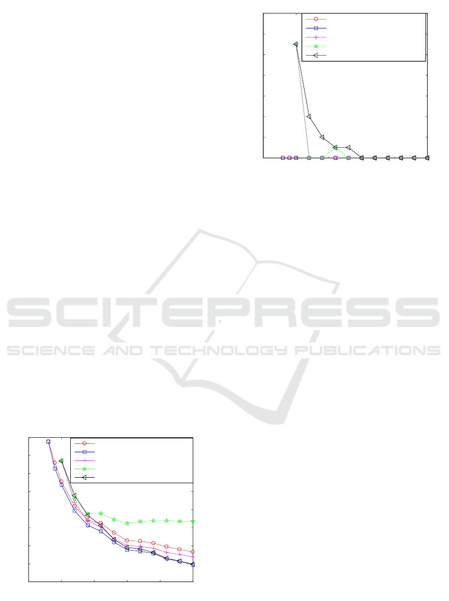
Figure 1: Relationship between number of image points
and RMS error.
Figure 2: Relationship between the number of image
points and the percentage of failures.
From Figure 1, we can see that with the
increasing of the number of image points, the RMS
errors of the sphere center calculated by the five
algorithms gradually decrease. Compared with the
traditional algorithms, the new method has an
advantage that the sphere center coordinates of the
target sphere can be calculated when there are only 3
or 4 image points. In addition, the normalized linear
curve fitting algorithm followed by center extraction
has the largest localization error of the sphere center,
and the new method followed by maximum
likelihood estimation has the smallest RMS error.
It can be seen from Figure 2 that the traditional
three algorithms have different percentages of
failures, but the new method proposed in this paper
has no case of failure. This shows that the new
method is more robust than the traditional
algorithms.
3.2 Relationship between the Depth of
the Sphere Center and RMS Error
The focal length of the camera is 2000 pixels. In the
camera coordinate system, we keep the ratio of the
X-axis coordinate, the Y-axis coordinate and the Z-
axis coordinate of the sphere center to be 2:3:4 and
uniformly select 10 sets of Z-axis coordinate, i.e. the
depth of sphere center, from 1 to 8 m. The sphere
radius is 0.005 m. The image points on the
projection ellipse are selected such that the distances
between adjacent points are approximately equal to
1 pixel. Gaussian white noise with zero mean and
standard deviation of 0.5 pixels is added to the
image points. The results are shown in Figure 3 and
Figure 4.
0 5 10 15 20 25
0.2
0.25
0.3
0.35
0.4
0.45
0.5
0.55
Number of image points
RMS error of sphere center
New method
New method + MLE
Ellipse direct fitting + center extraction
NDLT curve fitting + center extraction
MLE curve fitting + center extraction
0 5 10 15 20 25
0
0.1
0.2
0.3
0.4
0.5
0.6
0.7
Number of image points
Percentage of algorithm failures
New method
New method + MLE
Ellipse direct fitting + center extraction
NDLT curve fitting + center extraction
MLE curve fitting + center extraction
CTISC 2019 - International Conference on Advances in Computer Technology, Information Science and Communications
68
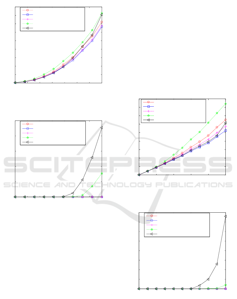
Figure 3: Relationship between the depth of sphere center
and the RMS error.
Figure 4: Relationship between the depth of the sphere
center and the percentage of failures.
It can be seen from Fig. 3 that, with the gradual
increasing of the depth of sphere center, the RMS
errors of the target sphere center calculated by the
five algorithms are approximately proportional to
the 2.5-th power of the depth. It is worth noting that,
during the increase of the depth of the sphere center,
the RMS error of the sphere center solved by the
normalized linear curve fitting algorithm followed
by center extraction is significantly larger than the
other four algorithms, and the smallest error is
obtained by using the new method followed by
maximum likelihood.
It can be seen from Fig. 4 that the new method
and the new method followed by maximum
likelihood improvement have no failure case. In
contrast, in the cases of large depths and
consequently small imaging ellipses, the traditional
algorithms have a large percentage of failures.
3.3 Relationship between Noise Level
and RMS Error
The focal length of the camera is 2000 pixels. In the
camera coordinate system, the target sphere center is
at (2, 3, 4)
T
m, and the sphere radius is 0.005 m. The
image points on the projection ellipse are selected
such that the distances between adjacent points are
approximately equal to 1 pixel. Gaussian white noise
with zero mean and standard deviation varying from
0 to 1.0 pixel is added to the image points. The
results are shown in Fig. 5 and Fig. 6.
Figure 5: Relationship between noise standard deviation
level and RMS error.
Figure 6: Relationship between noise standard deviation
level and percentage of failures.
1 2 3 4 5 6 7 8
0
0.2
0.4
0.6
0.8
1
1.2
1.4
1.6
1.8
Depth of sphere center
RMS error of sphere center
New method
New method + MLE
Ellipse direct fitting + center extraction
NDLT curve fitting + center extraction
MLE curve fitting + center extraction
1 2 3 4 5 6 7 8
0
5
10
15
20
25
Depth of sphere center
Percentage of algorithm failures
New method
New method + MLE
Ellipse direct fitting + center extraction
NDLT curve fitting + center extraction
MLE curve fitting + center extraction
0 0.2 0.4 0.6 0.8 1
0
0.1
0.2
0.3
0.4
0.5
0.6
0.7
0.8
0.9
Noise standard deviation level
RMS error of sphere center
New method
New method + MLE
Ellipse direct fitting + center extraction
NDLT curve fitting + center extraction
MLE curve fitting + center extraction
0 0.2 0.4 0.6 0.8 1
0
1
2
3
4
5
6
7
8
Noise standard deviation level
Percentage of algorithm failures
New method
New method + MLE
Ellipse direct fitting + center extraction
NDLT curve fitting + center extraction
MLE curve fitting + center extraction
Sphere Localization from a Minimal Number of Points in a Single Image
69

From Fig. 5 we can see that as the noise standard
deviation increases from 0 to 1 pixel, the RMS
errors of the sphere center calculated by the five
algorithms also increase linearly from the origin.
Comparing the RMS errors obtained by the five
algorithms, it can be seen that the RMS error of new
method followed by maximum likelihood estimation
is the smallest, while the normalized linear curve
fitting algorithm followed by center extraction has
the largest error under the same noise level.
It can be seen from Fig. 6 that in the process of
increasing the noise standard deviation, the new
method and the new method followed by maximum
likelihood estimation do not encounter failure case
in the calculation of the sphere center coordinates. In
contrast, the traditional three algorithms have
different percentages of failures when the noise level
is high.
4 CONCLUSIONS
When the target sphere radius and the camera
calibration matrix are known, the three-dimensional
coordinates of a sphere center can be calculated with
at least three measurement points on the image
ellipse by constructing and solving a set of quadratic
equations of the three variables in the sphere center
coordinates. Compared with traditional algorithms,
the new three-point method for calculating the
sphere center coordinates of the target sphere
proposed in this paper has several advantages. It can
work when the number of image points are less than
five. In addition, when the number of measurement
points increases to five or more, the proposed
method has a certain improvement in the location
accuracy and higher robustness than those of the
traditional algorithms. It can be seen from the
experimental results that the proposed method is
more practical than the traditional algorithms
especially when the image ellipse is small or the
noise level of the measuring point is high.
ACKNOWLEDGEMENTS
This work was supported in part by the National
Natural Science Foundation of China under Grants
No. 61703373, No. U1504604, No. 61873246, in
part by the Key research project of Henan Province
Universities under Grant 16A413017, and in part by
the Doctoral Scientific Research Foundation through
the Zhengzhou University of Light Industry under
Grant 2015BSJJ004.
REFERENCES
Fan, X., Hao, Y., Zhu, F., et al., 2016. Study on spherical
target identification and localization method for
robonuant. Manned Spaceflight, 22(03):375–380.
Geng, H., Zhao, H., Bu, P., et a1., 2018. A high accuracy
positioning method based on 2D imaging for spherical
center coordinates. Progress in Laser and
Optoelectronics.
Gu, F., Zhao, H., Bu, P., et al., 2012, Analysis and
correction of projection error of camera calibration
ball. Acta Optica Sinica, 32(12):209–215.
Hartley, R., Zisserman, A. 2004. Multiple view geometry
in computer vision, Cambridge University Press,
Second Edition.
Liu, S., Song, X., Han, Z., 2016. High-precision
positioning of projected point of spherical target center.
Optics and Precision, 24(8):1861–1870.
Shi, K., Dong, Q., Wu, F., 2012. Weighted similarity-
invariant linear algorithm for camera calibration with
rotating 1-D objects. IEEE Transactions on Image
Processing, 21(8):3806–3812.
Shi, K., Dong, Q., Wu, F., 2014. Euclidean upgrading
from segment lengths: DLT-like algorithm and its
variants. Image and Vision Computing, 32 (3):155–
168.
Shiu, Y. C., and Ahmad, S., 1989. 3D location of circular
and spherical features by monocular model-based
vision. IEEE International Conference on Systems,
Man and Cybernetics, Cambridge, MA, USA, 576–581.
Stewénius, H., Engels, C., Nistér, D., 2006. Recent
developments on direct relative orientation. ISPRS
Journal of Photogrammetry & Remote Sensing, 60:
284–294.
Sun, J., He, H., Zeng, D., 2016. Global calibration of
multiple cameras based on sphere targets. Sensors,
16(1):77.
Wei, Z., Sun, W., Zhang, G., et a1., 2012. Method for
finding the 3D center positions of the target reflectors
in laser tracking measurement system based on vision
guiding. Infrared and Laser Engineering, 41(4):929–
935.
Wong, K., Schnieders, D. and Li, S, 2008. Recovering
light directions and camera poses from a single sphere.
In Lecture Notes in Computer Science, 631-642.
Zhao, Y., Sun, J., Chen X., et al., 2014. Camera
calibration from geometric feature of spheres. Journal
of Beijing University of Aeronautics and Astronautics,
40(4): 558–563.
Zheng, X., Zhao, M., Feng, S., 2018. Two-step calibration
of probe tip center of planar target. Laser &
Optoelectronics Progress, 55(01):011201.
CTISC 2019 - International Conference on Advances in Computer Technology, Information Science and Communications
70
