Analysis of a Business Environment using Burstiness Parameter: The

Case of a Grocery Shop

Andreas Ahrens

, Ojaras Purvinis

, Detlef Hartleb

, Jelena Zaˇsˇcerinska

and Diana Miceviˇcien˙e

Hochschule Wismar, University of Technology, Business and Design, Wismar, Germany

Kaunas University of Technology, Kaunas, Lithuania

Centre for Education and Innovation Research, Riga, Latvia

Panev˙eˇzys University of Applied Sciences, Kaunas, Lithuania

Keywords:

Buyers’ Burstiness, Independent Event, Gap Processes, Binary Customer Behaviour, Burstiness Estimation,

Burstiness Measurement.

Abstract:

Nowadays, bursty business processes are part of our everyday life. Bursty business processes include such pro-

cesses as selling and buying, too. One of the contemporary challenges business environment has to deal with

is monitoring and controlling of burstiness in business processes. Monitoring and controlling of burstiness in

business processes often leads to the optimization of business processes. Validation of the model for analysing

buyers’ burstiness in business processes revealed the need in optimisation of the proposed model, as the elab-

orated model based on gap processes is complex for implementation, as well as for parameter estimation. For

optimization of the model for analysing buyers’ burstiness in business process, different levels of burstiness

in the process of buying are studied in this work. Different approaches to modelling buyers’ behaviours are

presented and evaluated in this work, too. The novel contribution of this work is based on the estimation of

burstiness. With the proposed solution the level of burstiness can be estimated by taking the mean value and

the standard deviation of a gap sequence into account, which always exists for a given sequence. As a practical

application, the cash register of a medium size grocery shop in Lithuania is analysed. The novelty of this paper

is given by the comparison of different approaches to measuring burstiness in real process data. Directions of

further research are proposed.

1 INTRODUCTION

Nowadays, bursty business processes or, in other

words, business environment are part of our everyday

life. Trafﬁc ﬂow in cities is bursty, data trafﬁc implies

to be of a bursty nature, customers’ ﬂow in shops are

not static, too, as shown in Fig. 1.

Bursty Business

Processes

Trac Flow Data Flow Customer Flow

Figure 1: A range of bursty business processes in everyday

life.

Bursty business processes include such processes

as selling and buying, as shown in Fig. 2. One of the

contemporary challenges business environment has

to deal with is monitoring and controlling of bursti-

ness in business processes. Monitoring and control-

ling of burstiness in business processes often leads

to the optimization of business processes. Burstiness

Bursty Business

Processes

Selling Buying

Figure 2: The inter-relationship between bursty business

processes as well as selling and buying.

has attracted a lot of attention starting with the mod-

elling of bursts or bundles of bit-errors in telecom-

munications. Such investigations have led to inten-

sive research for simulation models which are able to

take the bursty characteristic of bit-errors into account

such as (Gilbert, 1960) or (Elliott, 1963). Similar de-

pendencies can be found in data networks regarding

the characteristics of the trafﬁc (e.g. the temporal

intervals between consecutive data packets) (Kessler

Ahrens, A., Purvinis, O., Hartleb, D., Zaš

cerinska, J. and Micevi

cien

e, D.

Analysis of a Business Environment using Burstiness Parameter: The Case of a Grocery Shop.

DOI: 10.5220/0007977600490056

In Proceedings of the 9th International Conference on Pervasive and Embedded Computing and Communication Systems (PECCS 2019), pages 49-56

ISBN: 978-989-758-385-8

Table 1: Burstiness in different scientiﬁc ﬁelds.

Scientiﬁc ﬁeld Phenomenon of burstiness

Telecommunications Burstiness of bit-errors in data transmission

Economics Burstiness of crises

Natural sciences Burstiness of disasters or earthquakes

Logistics Burstiness of trafﬁc

Social media Burstiness of hot topic, keyword or event

Business Burstiness of workload

Business Burstiness of buyers

et al., 2003; Feldmann, 2000).

Furthermore, the phenomenon of burstiness was

revealed in a range of scientiﬁc ﬁelds such as eco-

nomics, natural sciences, logistics and business.

Tab. 1 demonstrates the phenomenon of burstiness in

a range of scientiﬁc ﬁelds.

In business, burstiness is based on visitor-buyer

relationship as illustrated in Fig. 3. The visitor-buyer

relationship implies binary customer behaviour such

as buying or not buying. A visitor becomes with the

probability p

a buyer (also referred as buyer prob-

ability) and remains with the probability (1 − p

) a

visitor.

Visitor Buyer

(1 − p

)

Figure 3: Visitor-Buyer Relationship.

However, these models do not take the concentra-

tion of buyers into account as highlighted Fig. 4.

x x - x x x - - x x x x x x - x x - - - - - - - - - - - -

- - - - - - - x x x x - x - - x x - - x x - - - - - - - -

- - - - - - - - - - - - - - - - - - - - - - - - - - - - -

- - - - - - - - - - - - - - - - - - - - - - - - - x x x x

- - - - - - - - - - - - - - - - - - - - - - - - - - - - -

- - - - - - - - - - - - - - - - - x x - - - - - - - - - -

- - - - - - - - - - - - - - - - - - - - - - - - - - - - -

- - - - - - - - - - - - - - x x x x - - - - - x - - x x -

- - - - - - - - - - - - - - - - - - - - - - - - - - - - -

- - - - x x x - - - - x x x - - - - - - - - - - - - - - -

- - - - - - - - - - - - - - - - - - - - - - - - - - - - -

- - - - - - - x x x - - - - - - - - - - - - - - - x x - -

- - - - - - - - - - - - - - - - - - - - - - - - - - - - -

x x x x x - - - - - - - - - - - x x - - x x x x x x - x -

- - - - - - - - - - - - - - - - - - - - - - - - - - - - -

- - - x x x x x x - - - - - - - - - - - - - - - - - - - -

Figure 4: Buyers’ burstiness (represented by ”x”) within a

sequence of shop visitor (represented by ”-”).

In (Ahrens and Zaˇsˇcerinska, 2017) a model for

analysing buyers’ burstiness in business processes has

been presented. The model shows that the process of

buying can be described by the buyers’ probability.

However, in order to be able to describe the bursty

nature of buyers a second parameter such as the buy-

ers’ concentration is needed.

The optimization of bursty business processes re-

quires, on the one hand, appropriate simulation mod-

els and, on the other hand, algorithms for estimating

burstiness in business processes in order to be able to

optimize process systems such as queuing at the cash

Optimization of business processes also depends

on a level of burstiness. Hence, an issue is the mea-

surement of burstiness. A couple of approaches to the

measurement of burstiness exist. The F (Fano) factor

as well as burstiness factor (1 − α) (also referred as

parameter in the present research) are widely used to

estimate a level of burstiness (Ahrens et al., 2019b).

In this work the level of burstiness in the process

of buying is studied. As a practical application, the

cash register of a medium size grocery shop in Lithua-

nia is analysed. The proposed solution of burstiness

estimation takes the mean value and the standard de-

viation of real data into account and avoids the com-

plex estimation of distribution or density functions.

The novelty of this paper is given by the compar-

ison of different approaches to measuring burstiness

in real process data.

The remaining part of this paper is organized as

follows: Section 2 introduces the theoretical basis for

modelling buyers’ behaviour. A mathematical model

for describing buyers’ burstiness via gap processes is

presented in Section 3. The estimation of burstiness

is introduced in Section 4. The associated results of

an empirical study of a medium size grocery shop in

Lithuania are discussed in Section 5. Finally, some

concluding remarks are provided in Section 6.

PECCS 2019 - 9th International Conference on Pervasive and Embedded Computing and Communication Systems

2 THEORETICAL BASIS

In this section the theoretical basis for describing

business processes with independent events of buy-

ers (i.e. the buyers appear independently from each

other) is given. In general, any process including

the process of buying in which binary decisions are

made can be described by gaps as illustrated in Fig. 5

(Ahrens et al., 2019a). Once the process is modelled

- x - - x - - x - - - x x - - - - x -

2 2 3 40

Figure 5: Modelling of the buying process by gaps (a buyer

(represented by ”x”) within a sequence of non-buying visi-

tors (represented by ”-”)).

by gaps, a gap distribution function u(k) deﬁning the

probability that a gapY between two buyers is greater

than or at least equal to a given number k, i.e.

u(k) = P(Y ≥ k) (1)

can be deﬁned within the following boundaries

u(0) = 1 and lim

k→∞

u(k) = 0 . (2)

Next to u(k) a gap density function v(k) deﬁning the

probability that a gap Y between two buyers is equal

to a given number k, i. e.

v(k) = P(Y = k) (3)

can be deﬁned. Taking v(k) into account, the function

u(k) results in

u(k) = v(k) + v(k + 1) + v(k+ 2) + · · · . (4)

For situations with independent events, i. e. buyers,

u(k) can be deﬁned, as a function of the buyers’ prob-

ability p

, as follows

u(k) = (1− p

)

. (5)

Equation (5) is well-known in probability theory for

independent events and is valid for any buyer proba-

bility p

. Therein, the probability of non-buying visi-

tors is deﬁned as

Number of Visitors - Number of Buyers

Number of Visitors

. (6)

With (5) the probability can be derived that ≥ k con-

secutive visitors are non-buying visitors.

By calculating the average gap length E(Y), the

interrelation between u(k) and p

becomes visible.

Here, we get

E(Y) + 1 =

. (7)

Calculating the sum of u(k), we receive

∞

∑

k=0

u(k) = u(0) +

∞

∑

k=1

u(k) = 1+

∞

∑

k=1

u(k) . (8)

With (4), the expression can be re-written as

∞

∑

k=0

u(k) = 1+

∞

∑

k=1

k· v(k) (9)

and the calculation of the average gap length E(Y)

becomes

E(Y) =

∞

∑

k=0

k· v(k) =

∞

∑

k=0

u(k) − 1 . (10)

The function v(k) can be decomposed with (4) as

v(k) = u(k) − u(k+ 1) . (11)

Combining (7) and (10), we get

∞

∑

k=0

u(k) =

. (12)

By taking (5) into account, (12) can be veriﬁed as fol-

lows

∞

∑

k=0

u(k) =

∞

∑

k=0

(1− p

)

1− (1− p

)

. (13)

Furthermore, deﬁning a given interval n with at least

one buyer, the block buyer probability p

(n) is for-

mulated as

(n) = 1− (1− p

)

(14)

and can be approximated for small p

as follows

(n) ≈ 1− (1− n p

) = n p

(15)

with

lim

n→∞

(n) = 1 . (16)

The block buyer probability p

(n) results from the

probability of having no buyers in a block of the

length n, deﬁned as (1− p

)

In a double-logarithmic representation the linear

relationship between log

(n)) and log

(n) be-

comes for p

(n) ≤ 1 evident. Here we get

log

(n)) = log

(n) + log

) . (17)

as it was conﬁrmed by practical measurements (Wil-

helm, 1976).

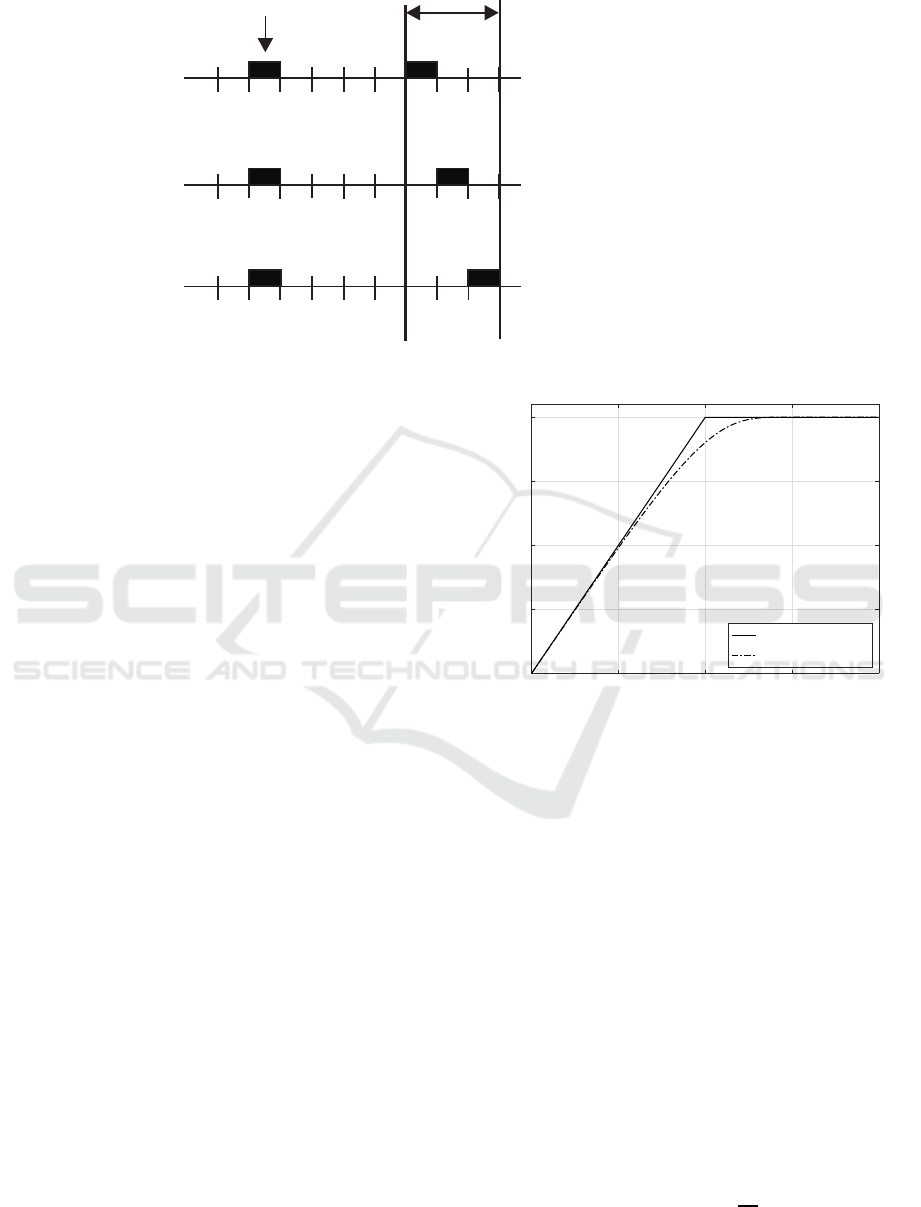
Furthermore, the block buyer probability p

(n)

can be calculated by taking the distribution function

u(k) into account as shown in Fig. 6 and results in

(n) = p

n−1

∑

k=0

u(k) (18)

Together with p

(n) = p

n, derived in (15), we get

n−1

∑

k=0

u(k) = n . (19)

The searched distribution u(k) can now be obtained

iteratively

Analysis of a Business Environment using Burstiness Parameter: The Case of a Grocery Shop

block interval

n = 3

P(1 buyer on position 1)

p u(0)

P(1 buyer on position 2)

p u(1)

P(1 buyer on position 3)

p u(2)

buyer

with p

Figure 6: Calculating the block-buyer probability p

(n) using the gap distribution function u(k).

n = 1 : u(0) = 1

n = 2 : u(0) + u(1) = 2

n = 3 : u(0) + u(1) + u(2) = 3

· · · : · · · = · · ·

n : u(0) + u(1) + · · · + u(n− 1) = n

and formulated as

u(k) = (k+ 1) − k = 1 . (20)

In order to fulﬁl (2) and (12), the function u(k), de-

ﬁned in (20), can be multiplied by

(1− p

)

≈ e

−p

·k

(21)

resulting in (5).

The resulting block buyers’ probability p

(n) is

highlighted in Fig. 7 when analysing the differences

in (15) and (18). The linear dependency between

log

(n)) and log

(n) for p

(n) ≤ 1 forms a ba-

sis for buyers’ simulation model.

3 DESCRIPTION OF BURSTY

BUSINESS PROCESSES

The bursty business processes have to consider that

the block buyer probability decreases for a given n as

the buyers become more and more concentrated. By

introducing a buyers’ concentration (1− α) as shown

in (Ahrens, 2000) and (Ahrens and Zaˇsˇcerinska,

2016) the block buyer probability can be approxi-

mated as

(n) = p

(22)

for any interval with p

(n) ≤ 1. In the double-

logarithmic representation we get

log

(n)) = α log

(n) + log

) . (23)

0 1 2 3 4

-2

-1.5

-1

-0.5

log

(n)) →

log

(n) →

Theory

Approximation

Figure 7: Approximated block buyer’s probability p

(n) as

a function of the interval length n for (1−α) = 0 at a buyer’s

probability of p

= 10

−2

with the parameter α deﬁning the gradient of the line.

Practically relevant buyers’ concentrations are in the

range of 0 < (1− α) ≤ 0.5, whereas a buyers’ concen-

tration of (1− α) = 0 describes the beforehand stud-

ied situation with independent buyers. Using (18), the

distribution function u(k) results in

n = 1 : u(0) = 1

n = 2 : u(0) + u(1) = 2

n = 3 : u(0) + u(1) + u(2) = 3

· · · : · · · = · · ·

n : u(0) + u(1) + · · · + u(n− 1) = n

and can be calculated as

u(k) = (k + 1)

− k

. (24)

In order to satisfy the condition

lim

k→∞

∑

κ=0

u(κ) =

(25)

PECCS 2019 - 9th International Conference on Pervasive and Embedded Computing and Communication Systems

(24) can be multiplied with the asymptote e

−β·k

with

lim

k→∞

−β·k

= 0 . (26)

By multiplying u(k) with the factor e

−β·k

, the param-

eter β has to be calculated in order to fulﬁl the condi-

tion

∞

∑

k=0

[(k+ 1)

− k

] · e

−β·k

. (27)

Taking the series expansion of the expression

(k+ ∆k)

= k

(1+

∆k+ ...) (28)

into account, the expression (24) simpliﬁes with ∆k =

1 to

(k+ 1)

− k

≈ α · k

α−1

. (29)

Using the integral instead of the sum, the following

equation has to be solved in order to determine the

parameter β. Here we get

U = α

∞

α−1

−β·k

dk =

α Γ(α)

, (30)

with the parameter Γ(·) describing the Gamma func-

tion. With the approximation

α Γ(α) ≈ 1 (31)

we get

∞

∑

k=0

[(k+ 1)

− k

] · e

−β·k

. (32)

Together with (27) the following approximation for

parameter β has been found

≈ β

. (33)

For bursty buying processes, the buyers’ gap distribu-

tion function results in

u(k) =

∞

∑

k=0

[(k+ 1)

− k

] · e

−β·k

. (34)

For independent buyers, i. e. α = 1, the parameter β

equals the buyer probability p

as derivedin section 2.

Fig. 8 demonstrates the buyers’ gap distribution

functions. With increasing buyers’ concentration

(1− α), the appearance of gaps of shorter lengths in-

creases whereas at the same time the probability of

longer gaps decreases.

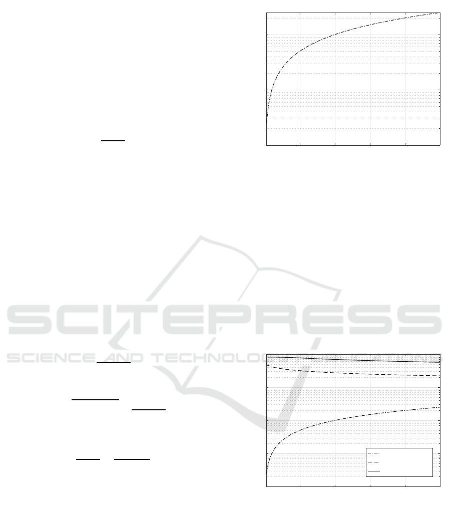
Fig. 9 shows the calculated block buyers’ proba-

bilities p

(n) as a function of the interval length n for

different parameters of the (1 − α) at buyers’ prob-

ability of p

= 10

−2

. With increasing buyers’ con-

centration, the buyers appear more and more concen-

trated and block buyer’s probability p

(n) decreases

for a given n as stated before. Furthermore, the lin-

ear dependence between log

(n) and log

(n))

becomes obvious for small n.

0.2

0.4

0.6

Probability →

gap length →

(1 − α) = 0.2

(1 − α) = 0.1

(1 − α) = 0.0

0 ... 10

11 ... 20

21 ... 30

Figure 8: Probability of different gap length for different

parameters of the (1− α) at a buyer’s probability of p

−2

0 1 2 3 4

-2

-1.5

-1

-0.5

log

(n)) →

log

(n) →

(1 − α) = 0.0

(1 − α) = 0.2

(1 − α) = 0.5

Figure 9: Approximated block buyer’s probability p

(n) as

a function of the interval length n for different parameters

of the (1− α) at a buyer’s probability of p

= 10

−2

4 ESTIMATION OF BURSTINESS

The practical evaluation of bursty buying processes

requires the calculation of the level of burstiness. A

possible approach can be deﬁned by the estimation of

the buyers’ concentration (1− α) as shown in (Ahrens

and Zaˇsˇcerinska, 2017). For this, the gap density

function v(k) has to be analysed. Analysing the prob-

ability that after a buyer, in the distance of zero an-

other buyer appears, i.e. v(0) = u(0) − u(1), the buy-

ers’ concentration (1 − α) can be analysed by taking

(34) into account. Here we ge with u(0) = 1

v(0) = 1 − u(1) = 1−

− 1) e

−β

. (35)

With the assumption of small beta the expression can

be simpliﬁed as follows

−β

≈ 1 for β ≪ 1 , (36)

and the parameter v(0) simpliﬁes to

v(0) ≈ 2 − 2

. (37)

From this equation, the buyers’ concentration (1− α)

is estimated as

(1− α) ≈ 1 − log

[2− v(0)] . (38)

Analysis of a Business Environment using Burstiness Parameter: The Case of a Grocery Shop

However, it requires the calculation of the gap density

function v(k). In comparison to (38), Goh & Barabasi

(Goh and Barab´asi, 2008) provided an alternative so-

lution for estimating burstiness in business processes.

In (Goh and Barab´asi, 2008) burstiness is deﬁned by

taking the mean value m (average gap length or aver-

age length of a time interval between two buyers) as

well as the standard deviation σ of the length of time

intervals or gaps into account. The deﬁnition by Goh

& Barabasi (Goh and Barab´asi, 2008) results in

B =

σ− m

σ+ m

. (39)

with −1 ≤ B ≤ 1.

Goh & Barabasi pointed out that B = 1 corre-

sponds to a bursty environment whereas B = 0 is re-

ferred to a neutral environment. Regular (periodic)

signals are described by negative parameters of B.

Analysing a buying process with independent buyers,

i. e. (1 − α) = 0, the gap distribution function u(k)

results in

u(k) = e

−p

·k

. (40)

Taking the gap density function v(k) = u(k)− u(k+1)

into account, the mean value m = E(Y) can be calcu-

lated as follows

m =

∞

∑

k=0

kv(k) =

∞

∑

k=0

k(e

−p

·k

− e

−p

·(k+1)

) (41)

and results in

m =

−p

1− e

−p

. (42)

Together with the standard deviation

σ =

E(Y

) − m

−p

1− e

−p

(43)

the parameter B results in

B =

σ− m

σ+ m

− 1

+ 1

. (44)

Fig. 10 shows the dependence of the parameter B

on the buyers’ probability p

. As shown by Goh &

Barabasi the parameter B is close to zero indicating

the independence of the buyers. However, the depen-

dence of the parameter B on the buyers’ probability

shows the weakness of the burstines deﬁnition as in-

dependent buyers’ scenarios are solely described by

the buyer probability. On the other hand the param-

eter B can be easily calculated for an empirically ob-

tained gap sequence.

Taking different parameters of the buyers’concen-

tration (1 − α) into account, Fig. 11 shows the ob-

tained values for the parameter B. As obtained by

computer simulations, the parameter B can be used

0.02 0.04 0.06 0.08 0.1

-4

-3

-2

→

B →

Figure 10: Dependence of the parameter B on the buyer’s

probability p

for independent buyers.

as an indicator regarding the level of burstiness. Ac-

cording to Fig. 11 a rough estimation leads to the fol-

lowing condition

B ≈ (1− α) . (45)

Unfortunately, the plot depicted in Fig. 11 shows that

the parameter B depends on the buyers’ probability p

and buyers’ concentration (1− α), i.e.

B = B(p

,(1− α))

is used as an indicator for the expected buyers’ con-

centration.

0.02 0.04 0.06 0.08 0.1

-4

-3

-2

-1

→

B →

(1 − α) = 0.0

(1 − α) = 0.2

(1 − α) = 0.5

Figure 11: Dependence of the parameter B on the buyer’s

probability p

for different parameters of the buyers’ con-

centration (1− α).

5 PRACTICAL APPLICATION

In real world business processes, the probability p

of visitor to buy a good as well as the correlation be-

tween buyers, described by the buyers’ concentration

(1− α), may be not available. The solution is to use

PECCS 2019 - 9th International Conference on Pervasive and Embedded Computing and Communication Systems

a statistical approach to estimate the buyers’ concen-

tration (1− α).

In this section the service of the buyers at the cash

analysed. In this example, the duration of the service

of the buyers at the cash register of a medium size

grocery shop in Lithuania is studied. The cash regis-

ter data collected contain the data about the operation

time, the amount of goods purchased, their codes, and

the prices paid by each buyer. The data collection was

carried out in June 2018. At that time 2575 buyers

were served.

Unfortunately, the cash registers do not record the

start time of the operation. Therefore, the service

duration time was not available from the database.

To cope with this problem we observed buyers’ ser-

vice durations with different quantities of goods (see

Tab. 2). It appeared, that the service duration t

de-

pends not only on the quantity of the goods, but also

on the type of goods, individual characteristics of the

buyer and other random factors, i. e. the dependence

is statistical.

Table 2: Duration of the service at the cash register.

Amount of Goods Service Time

g t

(ins)

3 44

1 18

10 30

1 11

18 61

1 37

The correlation coefﬁcient between g and t

equals

0,72 and the regression equation is given by

= 1,9g+ 22,8 . (46)

The equation yields that for one good about 1,9 sec-

onds and additionally about 22,8 seconds for each

buyer are required.

Knowing the quantity of goods and (46), the start

and end times of each buyer can be calculated. This

allows us to analyse the free time between two buyers’

service, if any. When it appeared that there was no

free time interval between two or several buyers’ ser-

vice, then the sequential service times were merged

into one continuous service time interval.

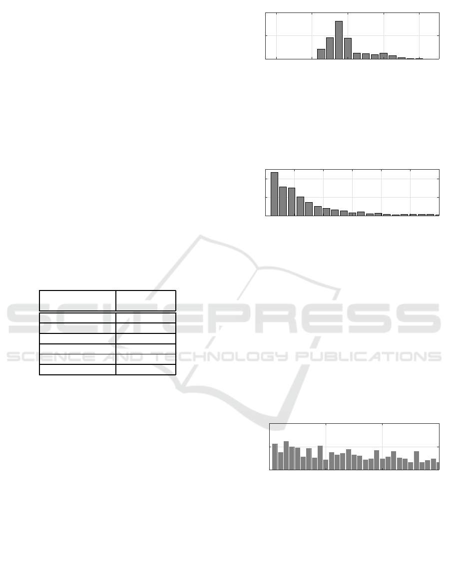
Therefore, it was possible to investigate service

duration times and time gaps between successive buy-

ers. It appeared that the average service duration is

37 seconds and the most frequent duration takes 32

seconds. The distribution of service duration time is

given in Fig. 12.

Similarly, the durationof free time intervals (gaps)

can be processed. The average free time interval (a

0 20 40 60 80

0.2

0.4

Probability →

t(ins) →

Figure 12: Distribution of service duration times.

gap) equals m = 234 s, i.e. 4 minutes and the stan-

dard deviation σ = 620 s. The histogram is given in

Fig. 13.

0 100 200 300 400 500 600

0.1

0.2

Probability →

t(ins) →

Figure 13: Distribution of free times of cash register

(grouped).

This histogram is different from the histogram of

service times. The frequencies of free times (gaps

of various lengths) are constantly decreasing while

it is not true for histogram of service times given in

Fig. 12.

The small mode of free time (gap lengths) and the

histogram of free times testiﬁes that the time gaps

between services usually are short. The histogram

of free times’ durations up to 30 seconds, i. e. half

minute, reveals that these durations are distributed

quite similarly (see Fig. 14.). One of the measures

0 10 20 30

0.05

0.1

Probability →

t(ins) →

Figure 14: Distribution of free time duration up to 30 sec-

onds.

of burstiness is the parameter B deﬁned in (39). Ap-

plying this formula to free times (gaps), it yields that

B = 0,45. Therefore, the free times between services

are quite bursty. On the other hand, the burstiness

level of free times up to 30 seconds states that this

process is close to neutral. The high burstiness of free

times during the whole month was determined by the

longer free time at the beginning and end of the shop

open time.

Analysis of a Business Environment using Burstiness Parameter: The Case of a Grocery Shop

6 CONCLUSIONS

In this work, on the example of the cash register of a

medium size grocery shop in Lithuania, different ap-

proaches to estimation burstiness are presented and

analysed. The proposed solution of burstiness esti-

mation takes the mean value and the standard devia-

tion into account and avoids the complex estimation

of distribution or density functions.

The discussed probabilistic models and their ap-

proximations of business processes can be evaluated

by the burstiness parameter B. It revealed, the bursti-

ness is positive, i. e. between neutral and bursty pro-

cess in the investigated case of a grocery shop in

Lithuania.

In real world business processes, the probability

of visitor to buy a good as well as the buyers’ con-

centration (1− α) may be not available. Nevertheless,

it is possible to process statistically the cash register

data. Usually the cash equipment just registers one

time moment of the service of the buyer and number

of goods and their codes in the basket, but not the

service duration. Therefore, the shop’s database does

not contain lengths of busy intervals and lengths of

free time intervals. The solution of the problem is an

additional observation of the cashier’s work, the reg-

istration of the number of goods in the buyer’s basket

and the service time of the basket. Then the regres-

sion equation between the number of goods in the

basket and service duration was derived. Using this

equation, it becomes possible to estimate the service

time lengths, to compute the free times and to apply

statistical analysis including calculation of burstiness

parameter.

Our plan on the future research is to investigate the

interrelationship between business process and visitor

decisions inﬂuenced by the behaviour of other visitors

and buyers.

ACKNOWLEDGEMENT

The authors of the present paper would like to thank

the grocery shop in Lithuania for supporting the mea-

surement campaign and providing the cash register

data.

REFERENCES

Ahrens, A. (2000). A new digital channel model suitable

for the simulation and evaluation of channel error ef-

fects. In Colloquium on Speech Coding Algorithms

for Radio Channels, London (UK).

Ahrens, A., Purvinis, O., and Zaˇsˇcerinska, J. (2019a).

Gap Distributions for Analysing Buyer Behaviour in

Agent-Based Simulation. In International Conference

on Sensor Networks (Sensornets), Prague (Czech Re-

public).

Ahrens, A., Purvinis, O., Zaˇsˇcerinska, J., Miceviˇciene, D.,

and Tautkus, A. (2019b). Burstiness Management for

Smart, Sustainable and Inclusive Growth: Emerging

Research and Opportunities. IGI Global.

Ahrens, A. and Zaˇsˇcerinska, J. (2016). Gap Processes for

Analysing Buyers’ Burstiness in E-Business Process.

In International Conference on e-Business (ICE-B),

pages 8–13, Lisbon (Portugal).

Ahrens, A. and Zaˇsˇcerinska, J. (2017). Analysing Buyers

Burstiness in E-Business: Parameter Estimation and

Practical Applications. In International Conference

on e-Business (ICE-B), Madrid (Spain).

Elliott, E. O. (1963). Estimates of Error Rates for Codes on

Burst-Noise Channels. Bell System Technical Journal,

42(5):1977–1997.

Feldmann, A. (2000). Characteristics of TCP Connection

Arrivals. In Park, K. and Willinger, W., editors, Self-

similar Network Trafﬁc and Performance Evaluation,

chapter 15, pages 367–399. Wiley.

Gilbert, E. N. (1960). Capacity of a Burst-Noise Channel.

Bell System Technical Journal, 39:1253–1265.

Goh, K.-I. and Barab´asi, A.-L. (2008). Burstiness and

Memory in Complex Systems. Exploring the Fron-

tiers of Physics (EPL), 81(4):48002.

Kessler, T., Ahrens, A., C., L., and Melzer, H.-D. (2003).

Modelling of connection arrivals in Ethernet-based

data networks. In 4rd International Conference on

Information, Communications and Signal Processing

and 4th IEEE Paciﬁc-Rim Conference on Multimedia

(ICICS-PCM), page 3B6.6, Singapore (Republic of

Singapore).

Wilhelm, H. (1976). Daten¨ubertragung (in German).

Milit¨arverlag, Berlin.

PECCS 2019 - 9th International Conference on Pervasive and Embedded Computing and Communication Systems