Two Cases of Study for Control Reconfiguration of Discrete Event
Systems (DES)
I. Tahiri
1,2 a
, A. Philippot
1b
, V. Carré-Ménétrier
1c
and A. Tajer
2d
1
Research Centre in Information and Communication and Technology (CReSTIC), URCA University, Reims, France
2
Electrical Engineering and Systems Control Laboratory (LGeCOS), UCA University, Marrakech, Morocco
Keywords: Control Reconfiguration, Supervisory Control Theory, Centralized Control, Distributed Control, Discrete
Event Systems, Timed Discrete Event Systems, Sensor Faults Detection, Manufacturing Systems.
Abstract: In this paper, we propose two cases of study for control reconfiguration of Discrete Event Systems. The main
contributions are based on a safe centralized and distributed control synthesis founded on timed properties. In
fact, if a sensor fault is detected, the controller of the normal behavior is reconfigured to a timed controller
where the timed information replaces the information lost on the faulty sensor. Finally, we apply our
contribution to a manufacturing system to illustrate our results and compare between the two frameworks.
1 INTRODUCTION
Nowadays, Manufacturing Systems (MS) are subject
to strong constraints induced by an uncertain
environment, changing and dominated by strong
international competition. This environment implies
that an MS is increasingly oriented towards a large
diversification of products manufactured in small and
medium series and not only towards a single type of
product.
The impact of this change in industry is reflected
by the need to have systems that can be able to adapt
to the production changes, to be flexible (Bordoloi,
Cooper, and Matsuo 1999), (Terkaj, Tolio, and
Valente 2009) and robust in order to meet the
diversity, the productivity (Rawat, Gupta, and Juneja
2018), the quality, the optimization of operating costs
and, finally, the reduction of failures risks requests.
We talk about factory of the future or industry 4.0 in
the sense that everything can be connected, simulated,
flexible and therefore reconfigured.
The respect of these constraints, which are
becoming more demanding, has led to a revolution in
the manufacturing field. This is manifested by the
increasingly massive use of powerful information
a
https://orcid.org/0000-0003-2203-2604
b
https://orcid.org/0000-0001-5229-9452
c
https://orcid.org/0000-0002-9576-9108
d
https://orcid.org/0000-0002-1528-7855
systems, especially, the increasing automation of
workshops and processes.
MS automation increases the productivity and the
competitiveness of companies engaged in the
manufactured goods production. Therefore, it is an
important economic issue. This automation requires
the development of methodologies including all the
system life cycle phases, from specification to
operation, in order to ensure a safe operating context
(Reniers 2017), (Tuptuk and Hailes 2018).
However, given the different parameters to be
considered in an MS, the latter becomes very complex
(Kul’ba et al. 2016). This complexity concerns both
the monitoring/ supervision as well as the control
part.
The Reconfigurable Manufacturing System
(RMS) concept invented by the University of
Michigan in 1999 (Y. Koren et al. 1999), is
considered as a new solution to gain competitiveness
and meet the requests of a constantly changing
market. In fact, designing an MS that can be
reconfigured (Yoram Koren and Shpitalni 2010)
accurately, quickly, and inexpensively according to a
market change offers a significant economic benefit
to manufacturing companies. The goal of an RMS is
to design systems with machines and controllers that
120
Tahiri, I., Philippot, A., Carré-Ménétrier, V. and Tajer, A.
Two Cases of Study for Control Reconfiguration of Discrete Event Systems (DES).
DOI: 10.5220/0007977301200129
In Proceedings of the 16th International Conference on Informatics in Control, Automation and Robotics (ICINCO 2019), pages 120-129
ISBN: 978-989-758-380-3
Copyright
c
 2019 by SCITEPRESS – Science and Technology Publications, Lda. All rights reserved

can meet the minimum cost and the new market
requirements that are characterized by diverse and
responsive needs. RMS also aim to adapt to changes
in both internal and external environments that
companies face.
The reconfiguration process is a reorganization
process of the system hardware and/ or software. The
objective of this reorganization is to be able to ensure
the production by making a compromise between the
objectives of production and the state of the system.
This reconfiguration process can be triggered by two
categories of events related to either products or
production resources.
A production change can be related to the
production nature, the quality or the number of
products. Indeed, in the manufacturing industry,
Flexible Manufacturing Systems (FMS) has been
designed to respond to the production of small or
medium series of products. This means that it may be
necessary on a given production horizon to start
manufacturing products that have not been scheduled.
This is only possible if the resources involved in
production do not operate at full load or if new
production resources can be committed. A change in
production can also be related to the quality of the
products. The requirement of a higher quality
compared to the one initially planned may require the
commitment of transformational resources able to
obtain it. It is the same principle for the quantity
whose requirements may vary during production.
Overall, these changes may lead to an addition or
removal of certain hardware resources related to the
set of those engaged in the current production.
On the other hand, a production resource state
change is characterized by two major events: failures
and repairs. In case of failures, the reconfiguration
process must first look for substituting the faulty
resource with another one. The goal in this context is
to use active or passive redundancies to recover the
failure. The two types of events that may trigger a
reconfiguration process are not necessarily
decoupled. In fact, a faulty resource can lead to a
change of production due to the impossibility of
finding the necessary production capacities in the
required time.
A reconfiguration process implementation
depends on two parameters: the trigger event and time
constraints exercising on the system when this event
occurs. Two complementary situations can be
considered: the case of a new production lunching
when the system is in a stop situation and the case of
a failure occurrence on a running system.
Most of the solutions proposed in the research work
as well as the practice ones are based on a material
redundancy to fill the failure of a system component.
Considering the technological development of the
components of manufacturing systems and their
complexity, this solution proves to be very expensive.
Therefore, in this work, we are interested to design
a reconfigurable control based on timed information of
a special class of MS: Discrete Event Systems (DES).
A DES (Cassandras and Lafortune 2008) is a dynamic
system whose state space is discrete. Its evolution is
governed by the occurrence of discrete events. These
physical events cause a change in the state of the
system.
The main idea is to design a reconfigurable control
able to adapt and exploit the services still available
offered by the system plant in case of a sensor fault
detection.
The reconfiguration process here consists on
leading the MS from its current state (CS) in the
normal behavior controller where the fault is
detected, thanks to the diagnosis, to a target state (TS)
in a faulty behavior controller in order to maintain the
MS functioning despite faults. The information lost
about a faulty sensor is replaced by a so-called time-
based estimator of its functioning (Tahiri et al. 2019).
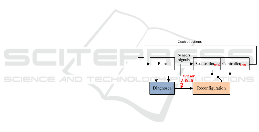
Figure 1: Control reconfiguration loop.
The control reconfiguration loop (figure 1) is based
on three elements: (1) The Supervisory Control Theory
principle (SCT) initiated by Ramadge and Wonham
(R&W) in (Ramadge and Wonham 1989). The SCT
aims at synthesizing a supervisor which ensures that
the behavior of a plant remains acceptable against the
specifications. (2) The diagnoser bloc that aims to
detect and isolate faults. Diagnosis is not the aim of this
paper, some related research works are given in (A.
Philippot and Carré-Ménétrier 2011), (Blanke et al.
2016), (Hélouët et al. 2014). In this work, we treat the
case of unobservable sensor faults that are defined by
a stuck-on/off of a sensor. (3) and finally, the
reconfiguration bloc which consists of taking the
decision to switch from a normal behavior controller to
a faulty one.
This paper is organized as follows: two cases for
control reconfiguration of DES are introduced in
section 2. The first case is based on a centralized
Two Cases of Study for Control Reconfiguration of Discrete Event Systems (DES)
121

control while the second one is founded on a
distributed control. In section 3, we illustrate our
results around a manufacturing system in addition to
a discussion on the application results. Finally, in
section 4, a conclusion of our presented work is
reported.
2 PROPOSED APPROACHES
2.1 Centralized Control
Reconfiguration of MS
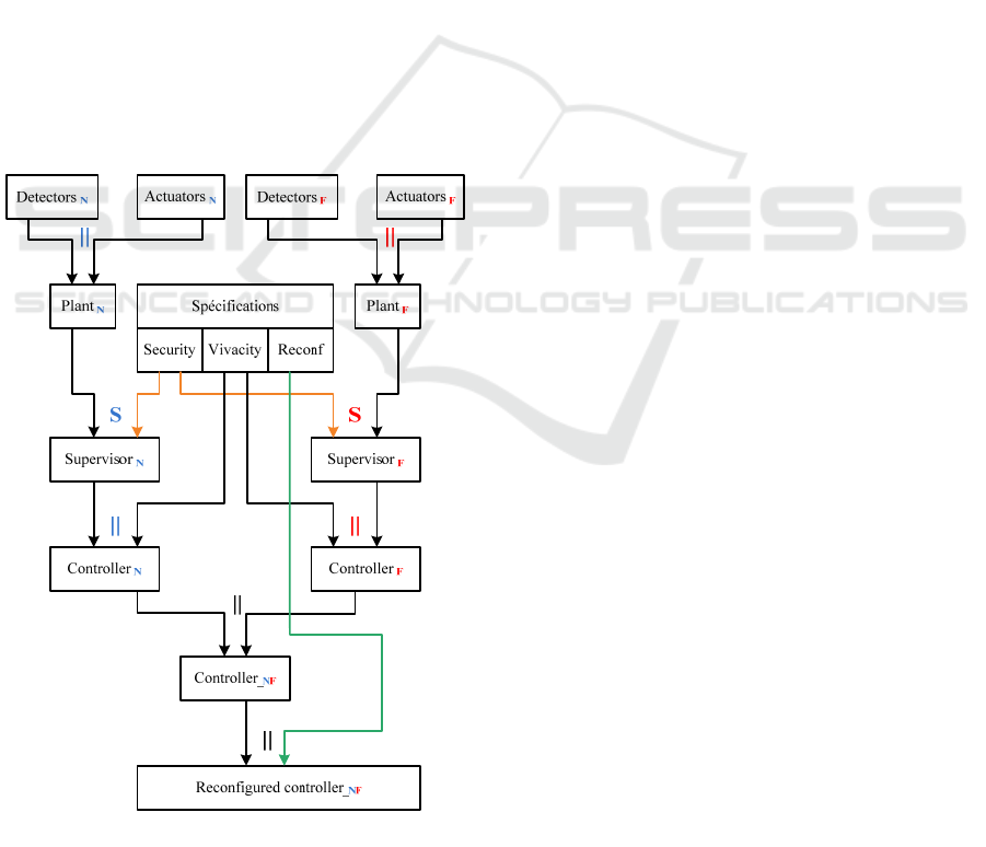
The first new framework proposed in this paper is a
centralized control reconfiguration of DES. The
method is based on defining two separate models of
the system plant. The first one describes the normal
behavior of the system and the second model
describes its faulty behavior where timed information
replaces each faulty sensor through a time-based
estimator (Tahiri et al. 2019). This, in order to
determine a centralized controller that manages the
two system’ behaviors as well as the switch between
them (figure 2).
Figure 2: Centralized control reconfiguration framework.
2.1.1 Defining the Plant_
N
and Plant_
F
Models
Defining the plant normal behavior model (plant_
N
)
is based on the practical model presented in
(Alexandre Philippot 2006). The main idea of this
practical model consists on devising the MS into
several plant elements (PE) and then defining a
detectors model (detectors_
N
) that describes the
normal behavior of all detectors constituting the
system’s PE, and an actuators model (actuators_
N
)
that describes the normal behavior of each actuator of
the MS with its associated detectors. The plant model
is given by the synchronization of these two models.
Formally, the “plant_
N
” model is defined by the
following automaton:
A_
N
= (Q_
N
, Σ_
N
, δ_
N
, q
0
_
N
, Q
m
_
N
) such as:
• Q_
N
is a finite set of all states of A_
N
.
• Σ_
N
is the set of events
• δ_
N
is the transition function. A transition is
defined by: δ_
N
(q_
N
, σ)=q’_
N
. σ is the occurrence of
an event of Σ_
N
.
• q
0
_
N
is the initial state of the automaton A_
N
,
such that q
0
_
N
∈Q_
N
.
• Q
m
_
N
is the set of marked states in A_
N
, such
that Q
m
_
N
⊆ Q_
N
.
The model presented above does not take into
account timed events which are the principle of the
faulty model. Therefore, determining the plant faulty
behavior model (plant_
F
) is based on an extension of
the practical model presented in (Alexandre Philippot
2006) where timed events are added. In a previous
work (Tahiri et al. 2019), we discussed a method to
include time to DES, we talk about Timed Discrete
Event Systems (TDES). A method where time is
presented through a clock and considered as an event,
which makes the modeling phase by Finite State
Machines (FSM) a simple task. In fact, the faulty
behavior (plant_
F
) or time-based estimator guaranties
the same normal behavior due to the replacement of
faulty sensors through the clocks that ensure their
functioning. The “plant_
F
” model is given by the
synchronization of the two-timed detectors model
(detectors_
F
) and actuators model (actuators_
F
).
Formally, the “plant_
F
” model is defined by the
following automaton:
A_
F
= (Q_
F
, Σ_
F
, δ_
F
, q
0
_
F
, Q
m
_
F
) such as:
• Q_
F
is a finite set of all states of A_
F
.
• Σ_
F
is the set of events, such as Σ_
F
= Σ
nT
∪ Σ
T
.
With: Σ
nT
is the set of non-timed events and Σ
T
is the
set of timed events such as: Σ
T
= C ∪ D with:
ICINCO 2019 - 16th International Conference on Informatics in Control, Automation and Robotics
122

C: Set of clocks, each clock is defined by an
activation and deactivation C= ↑ck
i
∪ ↓ck
i
D: Finite set of durations di associated to each
clock ck
i
, such as D= {d
1
, d
2
, …, d
i
}.
• δ_
F
is the transition function. A transition is
defined by: δ_
F
(q_
F
, σ)=q’_
F
. σ is the occurrence of
a timed event or not of Σ.
• q
0
_
F
is the initial state of the automaton A_
F
,
such that q
0
_
F
∈Q_
F
.
• Q
m
_
F
is the set of marked states in A_
F
, such
that Q
m
_
F
⊆ Q_
F
.
2.1.2 Defining Specifications
After having constituted the plant models of the
process, it is necessary to be able to integrate the
specifications information through a model of
specifications. It is the second step to achieve a
centralized control reconfiguration. The controller
establishes its specificities and represents the
behavior of normal operations of the process and
expresses safety constraints, what we must not do,
and liveness, what we must do, on the process.
Integrating the constraints of the specifications
consists of inhibiting actions and/ or arranging and
sequencing the execution of orders sent to the MS. A
constraint cannot cause additional actions in a model
but may express a restriction, or inhibition, of those
actions. The modeling of these constraints can be
carried out either by automatons or by logical
equations. The constraints can be applied either
globally to the whole process, or locally to each PE.
Our approach is based on obtaining a centralized
structure. Therefore, we apply both local and global
constraints modeled by FSM on the plant.
Each defined safety and/or liveness specification
on the normal behavior, its corresponding
specification in faulty behavior is determined too by
replacing the event associated to the sensor by its
corresponding clock.
The reconfiguration specifications are defined as
the constraints that allow the switch from normal
behavior to the faulty (timed) one when a faulty event
is detected. We define an automaton for each faulty
event. Afterward, all automata are synchronized to
obtain the automaton presenting the reconfiguration
constraints of the MS.
2.1.3 Defining Supervisors, Controllers and
Reconfigured Controller
The supervisor
_N
(resp supervisor
_F
) is obtained by
synthesizing the “plant_
N
” model (resp plant_
F
) with
its associated safety specifications. This step aims at
synthesizing a correct supervisor by construction,
which ensures that the behavior of a system remains
admissible compared to its specifications.
We note that the synchronization and/or the
synthesis in this work are applied through the
SUPREMICA software (Akesson et al. 2006).
The fourth step is to determine the controllers.
The controller_
N
(resp controller_
F
) is obtained
through synchronization of the supervisor_
N
model
(resp supervisor_
F
) with its associated liveness
specification. The resulting model describes the
desired behavior of the MS by the operator.
The supervisor should not be confused with the
controller. A supervisor here is a theoretical object,
which can inhibit, prohibit actions only and does not
take the initiative to trigger them. Thus, the
supervisor is not directly implementable.
Contrariwise, the controller allows both authorizing
and prohibiting actions and can be directly
implemented.
Afterward, to achieve a centralized control, the
two controller models “controller_
N
” and
“controller_
F
” are synchronized to obtain a global
model “controller_
NF
” which manages both normal
and faulty behaviors.
To make the controller_
NF
able of switching
between the two behaviors if a sensor fault is
detected, the reconfiguration specifications are
added. Therefore, a synchronization of the
“controller_
NF
” model with the reconfiguration
specification is needed. The resulting centralized
controller is called “reconfigured controller_
NF
”.
2.2 Distributed Control
Reconfiguration of MS
The idea behind proposing a second approach is the
fact that the first one discussed above presents a major
disadvantage which is the combinatorial explosion.
Indeed, studying complex MS under centralized
control is a complicated task to perform. Hence, it is
necessary to study the control reconfiguration with a
distributed architecture view.
The proposed framework for the distributed
control reconfiguration is presented in figure 3. It is
based in a first step on modeling the MS plant under
several plant elements. Then, two sets of
specifications are defined: local and global ones.
These specifications are integrated into several stages
of the control design in order to define the MS
different supervisors and both local and distributed
controllers. For each PE, two distributed controllers
are determined for normal and faulty behavior. For a
PLC implementation purpose, the distributed
controllers are interpreted into an IEC61131-3 PLC
Two Cases of Study for Control Reconfiguration of Discrete Event Systems (DES)
123

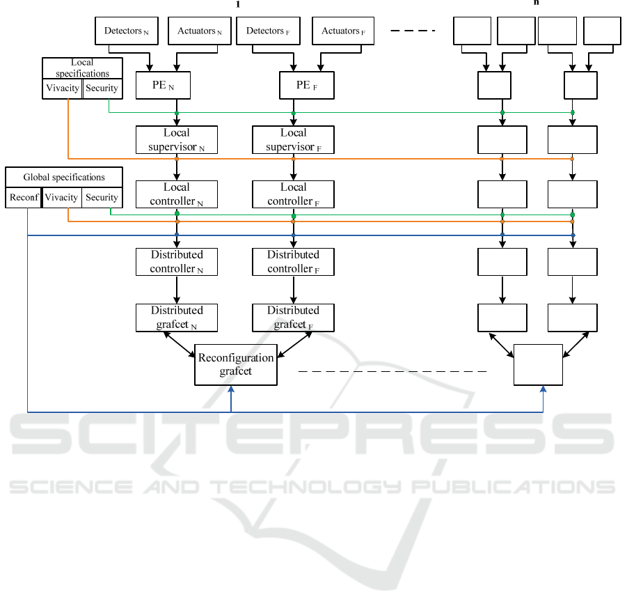
Figure 3: Distributed control reconfiguration framework.
programming language (SFC - Sequential Function
Chart language based on IEC60848 Grafcet tool).
Finally, the switch between the two controllers is
assured by the reconfiguration specifications which
are translated to Grafcet too.
2.2.1 Defining the PE_
N
and PE_
F
Models
A local specification can be defined by a logical
implication as given by the formula below:
 . = 0 (1)
Defining the two models of normal (PE_
N
) and
faulty (PE_
F
) behaviors of each PE of the MS is based
on the same modeling principle evoked in section
(2.1.1). Contrariwise, in this framework, we keep the
different practical models of each PE and we do not
synchronize them in order to achieve a distributed
control reconfiguration.
Let G denotes the set of PE models such as:
G= G_
N
∪ G_
F
with:
G_
N
=
⋃
A_



set of normal PE behaviors.
And
G_
F
=
⋃
A_



set of faulty PE behaviors.
n: is the number of PE constituting the MS.
2.2.2 Defining Specifications
To avoid the combinatorial explosion related to the
method proposed before in this paper, a specification
modeling method is proposed to overcome this
problem. Both local and global specifications are
presented by Boolean equations.
Such as “x” is a state of G state’s set and “y” is a
controllable event. The implication above means that
if x is true then y is forbidden.
A global specification of liveness or safety is
defined by a logical implication as given by the
expression below:
If c then {y = 0 else y = 1} (2)
Following the verification of the condition “c” if
it is true or not, the action “y” can be authorized (y =
1) or inhibited (y =0).
A condition “c” can belong to three different
categories (Qamsane, et al., 2016): A simple
condition using Boolean variables or functions, a
composed condition using a sequence of Boolean
variables or functions that precede each other, and a
ICINCO 2019 - 16th International Conference on Informatics in Control, Automation and Robotics
124

combined condition containing simple and composed
conditions such as: c ∈ ↑↓e
i
and/or c ∈ ↑↓d
i
.
Whereas, a reconfiguration specification (RS) is
defined by logical equations as follows:
RS:  

 

=1 
(: G
(

)
∗


)  (: G
(

)
∗
 
) (3)
Else If 

 

= 0 
(: G
(

)
∗




)  (: G
(

)
∗
 
)
Such as G
(

)
∗
is the grafcet associated to the normal
distributed controller and G
(

)
∗
is the grafcet
associated to the faulty distributed controller.
With 

is the Boolean variable associated to the step
“i” of G
(

)
∗
and 

its corresponding variable
associated to the step “ji” in G
(

)
∗
.
The expression
above means that if X
i
is active and a sensor fault is
detected, a switch to the faulty mode is requested by
forcing its grafcet G
(

)
∗
to start from the step 

and
deactivating the normal mode grafcet G
(

)
∗
.
2.2.3 Defining Supervisors, Controllers and
Reconfigured Controller
Local Synthesis Control.
In a previous work
(Tahiri et al. 2018), we proposed a new framework in
order to achieve a control synthesis. The approach is
based on an extension of the PE models. This
extension is generated by SUPREMICA software
(Akesson et al. 2006) through an Extended Finite
State Machine (EFSM) that contains guards, variables
and actions that can facilitate a compact
representation of a large and complex DES, unlike
FSM. The resulting automaton is noted {(A_
N
) curr}
for normal behavior and {(A_
F
) curr} for faulty
behavior.
To obtain the several local controllers for each PE,
we apply the synthesis of supervisory control using
SUPREMICA software between the {(A_
N
) curr} or
{(A_
F
) curr} models and the automaton presenting
the local specifications.
The local specification equation given in section
(2.2.2) is presented by an EFSM as shown in figure 4.
Each specification is composed of a single state
and a self-loop transition associated to the
controllable event “y” and the guard expressed by
{(A_
N
)_curr != x} or {(A_
F
)_curr != x}, which means
if the current state of (A_
N
) or (A_
F
) is different from
“x” then “y” is allowed.
The resulting automata of the control synthesis are
the local controllers of each PE and both normal and
faulty behaviors.
Figure 4: Local specifications modelling.
Global Synthesis Control. An MS running often
evokes the synchronism and parallelism between its
different PE. Thereby, a PE may depend on another
one to guarantee the desired behavior. Therefore,
communication between several PE is necessary. To
achieve that, a global control synthesis is needed to
obtain distributed controllers of normal behavior and
faulty one for each PE.
This synthesis consists first in aggregating the
local controllers as follows:
The untimed controllable events are merged into
macro-states. The states reached by controllable
events are associated in macro-states linked by
uncontrollable events (detectors events) or by timed
events {↑ck
i
, ↓ck
i
, d
i
}. If the local controller’s state is
associated to a rising edge of a controllable event,
then the order is authorized and belongs to the Ord
set. If it is associated to a falling edge of this event,
then the order is inhibited and belongs to the Inh set
The timed events ↑↓ck are merged
in macro-states
linked by uncontrollable events and timed events “d”.
If the state of the timed local aggregated controller by
the first aggregation reached by an event
corresponding to the clock' activation, then this event
belongs to a set noted A
CK
. If it is reached by an event
corresponding to the clock' deactivation, then this
event belongs to a set noted D
CK
. The self-loop
transition will be the transition that links the two
macro-states that contain the two sets (A
CK
and D
CK
).
The global specifications are added to the
resulting automata in order to obtain the different
distributed controllers.
An extract of a distributed controller is shown in
figure 5.
Two Cases of Study for Control Reconfiguration of Discrete Event Systems (DES)
125

(Ord: A
1
) if c
1
s
1
A
ck
: ck
1
D
ck
: ck
1
s
2
d
1
s
3
(Inh: A
2
) if c
2
Figure 5: Extract of distributed controller.
For an implementation purpose, the distributed
controllers and the reconfiguration specifications are
interpreted under a Grafcet language. A method of
this interpretation is given in (Tahiri et al. 2018) and
(Qamsane, et al., 2016).
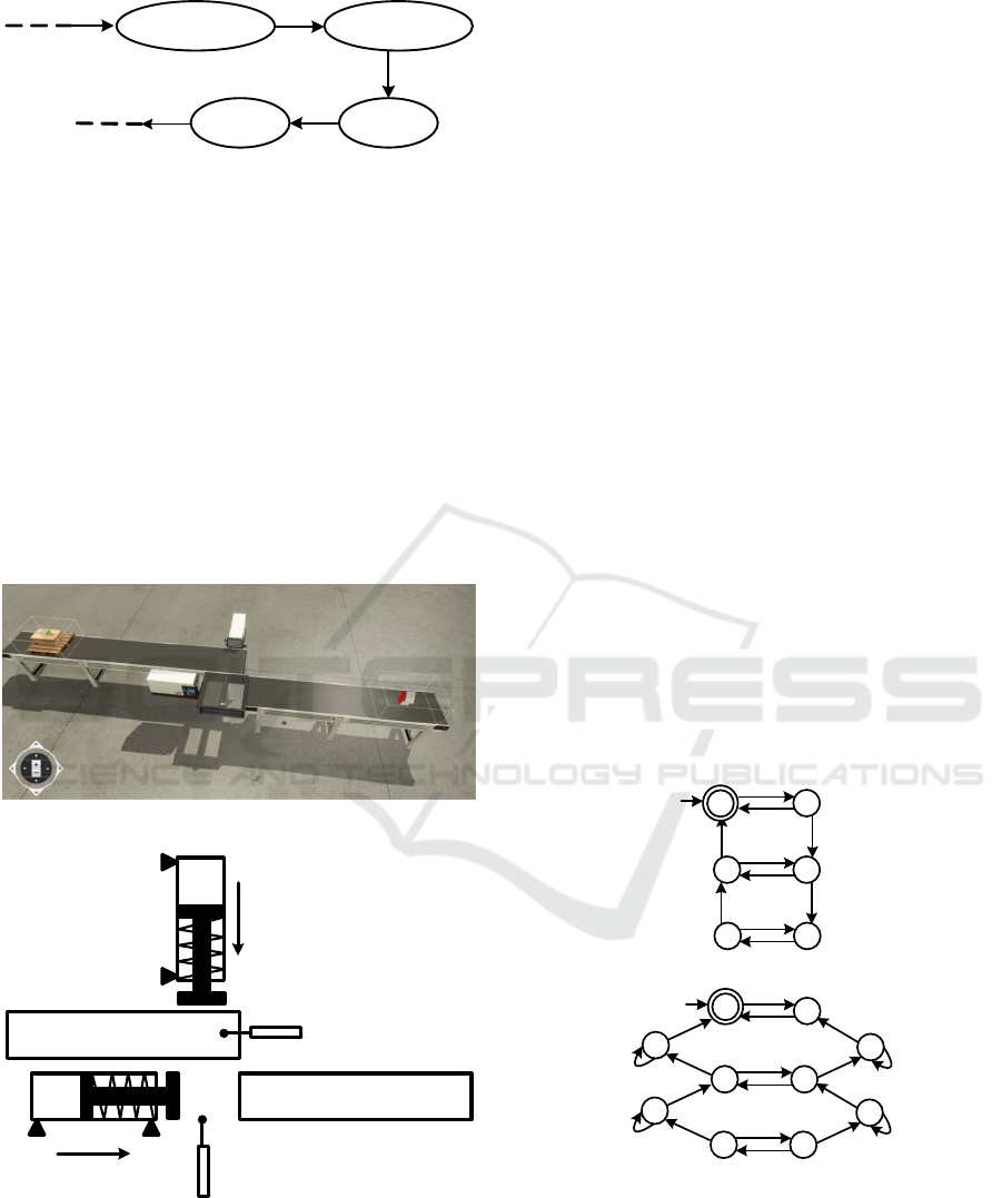
3 RESULTS AND DISCUSSION
The two approaches are applied to an MS (figure 6-b)
in order to reveal and evince the effectiveness of the
two contributions.
(a)
a
0
A
a
1
B
b
0
b
1
c
e
(b)
Figure 6: (a) The studied manufacturing system under
factory I/O, (b) The detailed studied manufacturing system.
This system is built using 3D FACTORY I/O
simulator (figure 6-a) (https://factoryio.com/). The
choice of this simulator is based on the fact that it
gives us the possibility to create our own system,
while allowing a generation of different faults for
either actuators or sensors.
The studied example consists of two pushers A
and B presented by two monostable single effect
cylinders with their associated limit sensors ({a0, a1}
for A and {b0, b1} for B). Two conveyor belts to
transport boxes in front of A, and to evacuate boxes
to the stock. Two position sensors: c (resp. e) to detect
boxes in front of A (resp. B). And finally, a start push
button (dcy).
In this paper, we study the behavior of pushers A
and B and we ignore the two conveyor belts. For a
distributed structure, the PE modeling is achieved
according to the model presented in section (2.2.1).
For each pusher, we determine the normal and faulty
behaviors (figure 7) and (figure 8).
The models are realized by the help of
SUPREMICA software. A falling edge refers in
models to “down” and a rising edge refers to “up”. In
case of a0 fault detection, the sensor deactivation is
replaced by the clock ck1 and the activation by the
clock ck2. It is the same for a1 (clock ck3 for a1
activation and clock ck4 for a1 deactivation), for b0
(clock ck6 for b0 activation and clock ck5 for b0
deactivation) and b1 (clock ck7 for b1 activation and
clock ck8 for b1 deactivation).
(a)
1
25
↑A
↑A
↓A
↓A
34
↓A
↑A
↓a
0
↑a
0
↑a
1
↓a
1
00
1
↑A
↓A
56
↓A
↑A
4
↑ck
3
↓ck
1
7
↑ck
4
↓ck
4
d
3
d
4
00
(b)
38
↓A
↑A
2
↑ck
3
↑ck
1
9
↑ck
2
↓ck
2
d
1
d
2
Figure 7: (a) normal and (b) faulty behaviors of pusher A.
ICINCO 2019 - 16th International Conference on Informatics in Control, Automation and Robotics
126

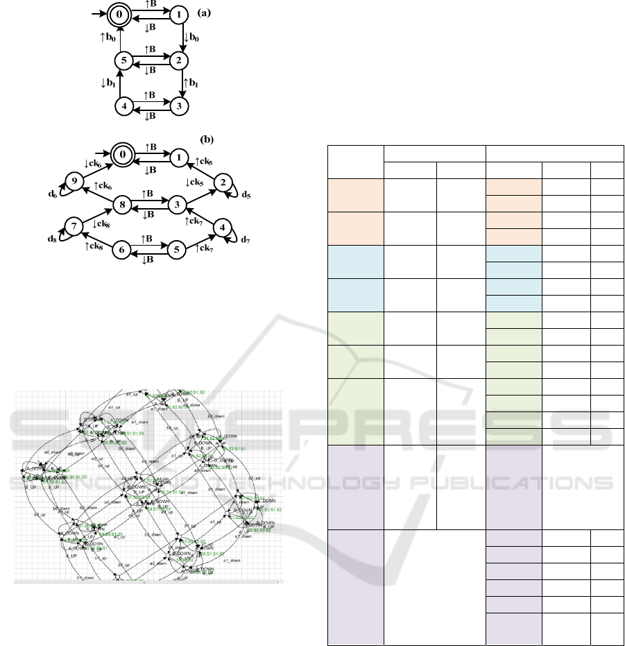
Figure 8: (a) normal and (b) faulty behaviors of pusher B.
While the centralized approach consists of defining the
two global models of normal and faulty behavior. To obtain
the normal plant modeling, the two normal models of
pushers A and B are synchronized. The resulting automaton
is given in figure 9.
Figure 9: Extract of normal behavior of A and B.
In the same way, we obtain the faulty behavior of
A and B
The normal behavior model is constituted by 36
states and 120 transitions. While the faulty behavior
model is constituted by 100 states and 360 transitions.
In this stage of the centralized framework design, we
observe the high number of states compared to the
distributed approach.
The safety constraint of this MS is defined as
follows: Do not send the exit orders of both cylinders
A and B at the same time.
It is possible to define as liveness constraints the
following specifications:
* Allowing the exit order of a pusher can only be
realized if the cylinder is in a return position (a0/b0).
* The exit order of cylinder B can only be
performed after the output of cylinder A.
Applying these different specifications in
different stages of the control reconfiguration design
for both contributions allows us to compare the two
approaches in different stages too as shown in table 1.
Table 1: Comparative table of the two proposed
approaches.
Centralized app Distributed app
States Trs States Trs
PO
N
36 120 PE
NA
6 10
PE
NB
6 10
PO
F
100 360 PE
FA
10 18
PE
FB
10 18
Sup
N
27 72 Sup
NA
6 10
Sup
NB
6 10
Sup
F
72 240 Sup
FA
10 18
Sup
FA
10 18
Ctrl
N
27 46 Ctrl
LNA
6 6
Ctrl
LNB
6 6
Ctrl
F
75 191 Ctrl
LFA
10 14
Ctrl
LFB
10 14
Ctrl
NF
675 2521 Ctrl
DNA
4 4
Ctrl
DNA
4 4
Ctrl
DFA
4 4
Ctrl
DFB
4 4
Ctrl
reconf
172800
52800
Does not
exist because
the control is
distributed
Grafcet
of
“Ctrl
reconf”
The control
Grafcet is
difficult to obtain
because of the
higher states
number of the
reconfigurable
controller
G
NA
5 5
G
NB
6 7
G
FA
5 5
G
FB
6 7
G
RA
7 8
G
RB
7 8
Trs refers to the number of transitions.
Sup
N(A/B)
refers to the supervisor of the normal
behavior of pusher A/B.
Sup
F(A/B)
refers to the supervisor of the faulty
behavior of pusher A/B.
Ctrl
LN(A/B)
refers to the local controller of the
normal behavior of pusher A/B.
Ctrl
LF(A/B)
refers to the local controller of the faulty
behavior of pusher A/B.
Ctrl
DN(A/B)
refers to the distributed controller of the
normal behavior of pusher A/B.
Ctrl
DF(A/B)
refers to the distributed controller of the
faulty behavior of pusher A/B.
Two Cases of Study for Control Reconfiguration of Discrete Event Systems (DES)
127

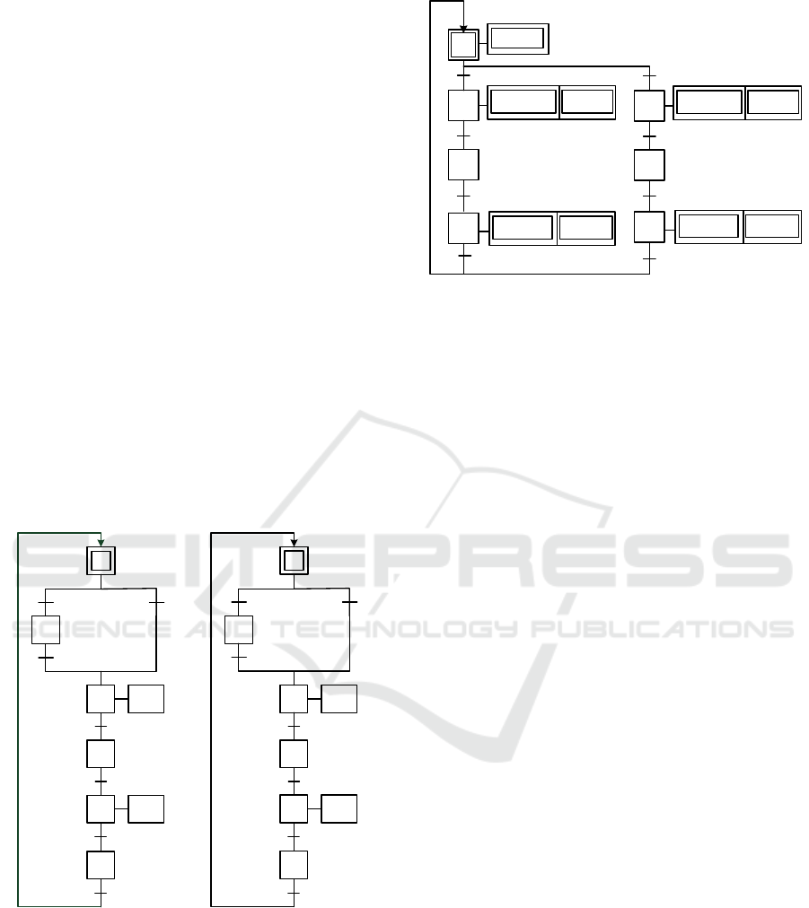
G
N(A/B)
refers to the Grafcet corresponding to the
distributed controller of the normal behavior of
pusher A/B (figure 10).
G
F(A/B)
refers to the Grafcet corresponding to the
distributed controller of the faulty behavior of pusher
A/B (figure 10).
G
R(A/B)
refers to the reconfiguration Grafcet
(figure 11) allowing the switch from G
N(A/B)
to G
F(A/B).
By analyzing the table above, we deduce that the
centralized approach for a control reconfiguration
presents a combinatorial explosion. This is due to the
use of the classic SCT in one hand. And on the other
hand, to the centralized structure, the second
drawback is the ability to implement the resulting
models. In fact, it is to complicate to interpret the
resulting exploded models into a language of PLC
programming. Moreover, despite that the MS
proposed in this paper is a simple system constituted
of two pushers, the corresponding reconfigured
controller is given under a large size of states and
transitions, which proves that obtaining the one
corresponding to a complex system is a difficult task.
Hence, the distributed approach solved the issues
related to the first contribution.
0
1
d_c c
d9/ X1
2
3
A:=1
4 A:=0
↑a1
↓a0
↓a1
↑a0
5
10
11
d_c c
d9/ X11
12
13
A:=1
14 A:=0
d3/X13
d1/X12
d4/X14
d2/X15
15
(a)
(b)
Figure 10: (a) G
NA
and (b) G
FA
Grafcets.
Let “d_↓a0” be the fault detected on the sensor a
0
deactivation, and “↑a0” the fault detected on the sensor a
0
activation. The reconfiguration Grafcet for pusher A is
given in figure 11.
Figure 11: The reconfiguration Grafcet of pusher A.
4 CONCLUSIONS
Responding to the operational safety issues in the
field of systems’ control, the implementation of
formal methods is necessary. In this context, it is
important to monitor the MS and to offer an
alternative solution to maintain the production. Thus,
a control reconfigure-tion of MS is required. For this
aim, this paper has presented two new frameworks,
the first one is based on a centralized control which
we proved its low performance by an application on
a transfer system. The second one is focused on a
distributed control which comes to face out the
problems related to the centralized approach. The key
advantage of a distributed control reconfiguration
approach is the use of distributed control that in the
one hand avoid the combinatorial explosion recurrent
in the centralized, approaches. On the other hand, it
allows the reconfiguration of the only faulty PE
without reconfiguring all the system’s control. In
addition, to replace the faulty sensor events by timed
events that ensure the same behavior avoid the use of
the redundant element.
Our perspectives include the verification of the
timed synthesis control proposed for the faulty or
reconfigured mode. Also, we intend to develop the
axis of reconfiguration of DES. In fact, a controller
can be reconfigured due to a system’s configurations
change or to the specifications change according to
the operator request. Feedback information for the
operator on the faulty sensor repair can be taken into
account. Therefore, this information will allow the
switch from faulty behavior to the normal one. This
could give some insights to be applied to a real MS
(http://www.univ-reims.fr/meserp/cellflex-.0/cellflex
-4.0,9503,27026.html) existing in our laboratory to
improve the proposed work in future research.
101
G
(FA)
{12}
X2 . d_↓a0
100
G
(NA)
{ }
G
(FA)
{ }
102
X12
X13
104
G
(FA)
{15}
X5 . d_↑a0
G
(N)
{ }
105
X15
X10
103
G
(NA)
{ 3 } G
(FA)
{ }
X3
106
G
(NA)
{ 0 } G
(FA)
{ }
X0
ICINCO 2019 - 16th International Conference on Informatics in Control, Automation and Robotics
128

REFERENCES
Akesson, K., M. Fabian, H. Flordal, and R. Malik. 2006.
“Supremica - An Integrated Environment for
Verification, Synthesis and Simulation of Discrete
Event Systems.” In 2006 8th International Workshop
on Discrete Event Systems, 384–85.
https://doi.org/10.1109/WODES.2006.382401.
Blanke, Mogens, Michel Kinnaert, Jan Lunze, and Marcel
Staroswiecki. 2016. “Introduction to Diagnosis and
Fault-Tolerant Control.” In Diagnosis and Fault-
Tolerant Control, 1–35. Springer, Berlin, Heidelberg.
https://doi.org/10.1007/978-3-662-47943-8_1.
Bordoloi, Sanjeev K., William W. Cooper, and Hirofumi
Matsuo. 1999. “Flexibility, Adaptability, and
Efficiency in Manufacturing Systems.” Production and
Operations Management 8 (2): 133–50.
https://doi.org/10.1111/ j.1937-5956.1999.tb00366.x.
Cassandras, Christos G, and Stéphane Lafortune. 2008.
Introduction to Discrete Event Systems. Second
Edition. New York. //www.springer.com/us/book/
978038733 3328.
Hélouët, Loïc, Hervé Marchand, Blaise Genest, and
Thomas Gazagnaire. 2014. “Diagnosis from
Scenarios.” Discrete Event Dynamic Systems 24 (4):
353–415. https://doi.org/10.1007/s10626-013-0158-2.
Koren, Y., U. Heisel, F. Jovane, T. Moriwaki, G. Pritschow,
G. Ulsoy, and H. Van Brussel. 1999. “Reconfigurable
Manufacturing Systems.” CIRP Annals 48 (2): 527–40.
https://doi.org/10.1016/S0007-8506(07)63232-6.
Koren, Yoram, and Moshe Shpitalni. 2010. “Design of
Reconfigurable Manufacturing Systems.” Journal of
Manufacturing Systems 29 (4): 130–41.
https://doi.org/10.1016/j.jmsy.2011.01.001.
Kul’ba, V., L. Busk Kofoed, D. Kononov, and O. Zaikin.
2016. “Scenario Research of Complex Manufacturing
Systems’ Vulnerability.” IFAC-PapersOnLine, 8th
IFAC Conference on Manufacturing Modelling,
Management and Control MIM 2016, 49 (12): 372–77.
https://doi.org/10.1016/j.ifacol.2016.07.633.
Philippot, A., and V. Carré-Ménétrier. 2011. “Methodology
to Obtain Local Discrete Diagnosers: Submission for
Special Session on Diagnosis of DES: Application on a
Benchmark.” In 2011 3rd International Workshop on
Dependable Control of Discrete Systems, 47–52.
https://doi.org/10.1109/DCDS.2011.5970317.
Philippot, Alexandre. 2006. “Contribution Au Diagnostic
Décentralisé Des Systèmes à Événements Discrets:
Application Aux Systèmes Manufacturiers.” Reims,
France: Reims champagne Ardenne University.
Qamsane, Yassine, Abdelouahed Tajer, and Alexandre
Philippot. 2016. “A Synthesis Approach to Distributed
Supervisory Control Design for Manufacturing
Systems with Grafcet Implementation.” International
Journal of Production Research, September.
http://tandfonline.
com/doi/abs/10.1080/00207543.2016.1235804.
Ramadge, P. J. G., and W. M. Wonham. 1989. “The Control
of Discrete Event Systems.” Proceedings of the IEEE
77 (1): 81–98. https://doi.org/10.1109/5.21072.
Rawat, Govind Singh, Ashutosh Gupta, and Chandan
Juneja. 2018. “Productivity Measurement of
Manufacturing System.” Materials Today:
Proceedings, International Conference on Processing
of Materials, Minerals and Energy (July 29th – 30th)
2016, Ongole, Andhra Pradesh, India, 5 (1, Part 1):
1483–89. https://doi.org/10.1016/j.matpr.2017.11.237.
Reniers, G. 2017. “On the Future of Safety in the
Manufacturing Industry.” Procedia Manufacturing,
Manufacturing Engineering Society International
Conference 2017, MESIC 2017, 28-30 June 2017, Vigo
(Pontevedra), Spain, 13 (January): 1292–96.
https://doi.org/10.1016/j.promfg.2017.09.057.
Tahiri, Imane, Alexandre Philippot, Véronique Carré-
Ménétrier, and Abdelouahed Tajer. 2018. “Timed
Synthesis Approach for Tolerant-Fault Control of
Discrete Event Systems (DES)”. International
Conference on Control, Automation and Diagnosis
(ICCAD'18). 19-21 March 2018, Marrakech-Morocco.
Tahiri, Imane, Alexandre Philippot, Véronique Carré-
Ménétrier, and Abdelouahed Tajer. 2019. “Time-Based
Estimator for Control Reconfiguration of Discrete
Event Systems (DES).” the International Conference on
Control, Decision and Information Technologies
(codit'19). 23-26 April 2019; Paris-France.
Terkaj, Walter, Tullio Tolio, and Anna Valente. 2009. “A
Review on Manufacturing Flexibility.” In Design of
Flexible Production Systems: Methodologies and
Tools, edited by Tullio Tolio, 41–61. Berlin,
Heidelberg: Springer Berlin Heidelberg. https://doi.
org/10.1007/978-3-540-85414-2_3.
Tuptuk, Nilufer, and Stephen Hailes. 2018. “Security of
Smart Manufacturing Systems.” Journal of
Manufacturing Systems 47 (April): 93–106.
https://doi.org/10.1016/j.jmsy.2018.04.007.
Two Cases of Study for Control Reconfiguration of Discrete Event Systems (DES)
129