Development of Spatial Quality Control Method for Temperature
Observation Data using Cluster Analysis
Yunha Kim, Nooree Min, Hannah Lee, Mi-Lim Ou, Sanghyeon Jeon and Myung-jin Hyun
National Climate Data Center, Korea Meteorological Administration, South Korea
Keywords: Temperature, Cluster Analysis, Meteorological Observation, Quality Control, Spatial Checking.
Abstract: In the National Climate Data Center of Korea Meteorological Administration, quality control methods of
meteorological observations are applied to identify erroneous observation values. The type of quality control
methods we have been using is to check the value from one station, either instantly or temporally. The spatial
checking methods that find errors by comparing values of several stations at a time are difficult to apply
because calculating the threshold using a large amount of observations is time consuming and various
conditions for applying are required. In this study, we develop a new spatial checking method for temperature
observation data using cluster analysis for meteorological observations that can be performed fast and
effective in clarifying errors that have not been discovered.
1 INTRODUCTION
Data quality control of meteorological observations is
the process of examining data to detect missing
values and errors in order to eliminate errors and
provide high-quality data for users (WMO, 2013).
The National Climate Data Center (NCDC) of the
Korea Meteorological Administration (KMA) has
applied quality control methods automatically to
observation data collected from more than 600
stations. The methods that have been applied to
temperature observation data are single station checks
using instant observation or one time series data from
one station, e.g., range checks, step checks and
consistency checks.
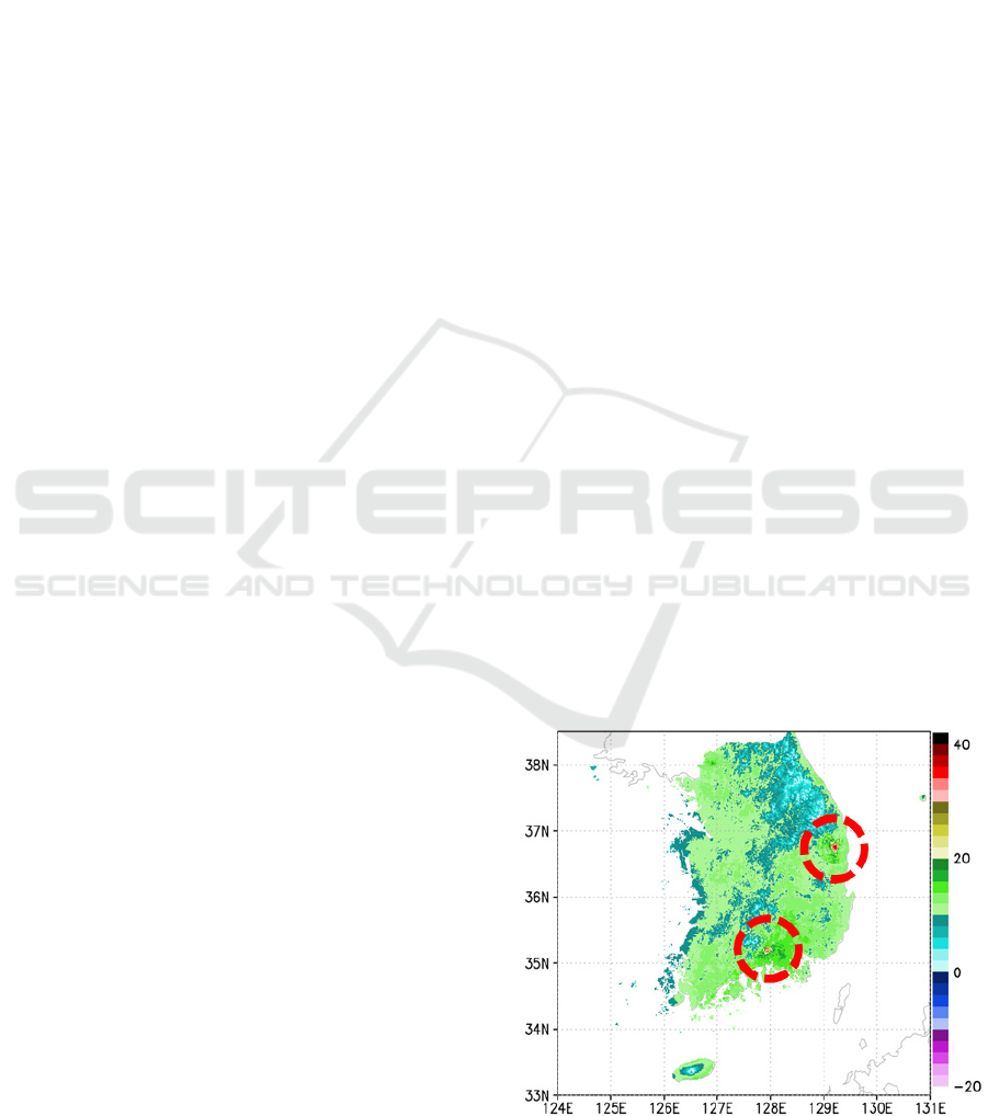
Figure 1 shows the maximum temperature
distribution in South Korea on March 8, 2003 using
the MK (Modified Korean)-PRISM (Parameter-
elevation Regressions an Independent Slopes Model)
(Kim et al., 2012). The circled parts in Figure 1
indicate points where the temperature difference with
the surrounding points is approximately 15 to 20 °C.
The values of the points are likely to be errors. The
single station checking methods currently used
cannot detect this type of errors because the methods
have the same spatial error-determination criteria;
however, the spatial checking method can be used to
find erroneous data by comparing observation values
at several stations. Several spatial tests have been
reported in the literature, such as the Cressman
scheme (Cressman, 1959) and Barnes scheme
(Barnes, 1964). However those spatial checks have
not been used in the NCDC because it is time
consuming to calculate the threshold to be compared
with the actual data value and various conditions are
required. Therefore, we develop a new spatial quality
control method for temperature observations using
clustering analysis for meteorological stations that
can quickly find errors by comparing values at
various stations.
Figure 1: Maximum temperature distribution in South
Korea on March 8, 2013.
364
Kim, Y., Min, N., Lee, H., Ou, M., Jeon, S. and Hyun, M.
Development of Spatial Quality Control Method for Temperature Observation Data using Cluster Analysis.
DOI: 10.5220/0007965703640368
In Proceedings of the 8th International Conference on Data Science, Technology and Applications (DATA 2019), pages 364-368
ISBN: 978-989-758-377-3
Copyright
c
2019 by SCITEPRESS – Science and Technology Publications, Lda. All rights reserved
2 PROCESSING OUTLINE
The development of spatial quality control method is
divided into two stages: Cluster analysis for
meteorological stations and setting of error
determination criteria.
2.1 Cluster Analysis
This section describes the result of Kim et al. (2017)
that includes the cluster analysis by month for
meteorological observation stations using the gridded
data of numerical weather prediction.
2.1.1 Grid Data Clustering by Month
For cluster analysis, Kim et al. (2017) use gridded
data from numerical model instead of meteorological
observation data from stations to reflect the climate
characteristic of South Korea evenly. The numerical
model data used are the KLAPS model data for 2006–
2014. The model data are 5km 5km gridded
observations in time unit (Kim et al., 2013). The grid
points corresponding to the land and coast of South
Korea are used for analysis, and the number of grid
points used is 20,044. Daily temperature datasets
calculated by averaging hourly data of the numerical
model are used as input datasets for cluster analysis.
The methods used in the cluster analysis are the
Ward method and K-means method. The Ward
method is a hierarchical cluster analysis method
considering the incremental sum of squares in the
cluster and the intersection of squares between the
clusters (Ward, 1963; Murtagh and Legendre, 2014).
The K-means method, which is a non-hierarchical
cluster analysis method, requires that the number of
clusters be defined in advance and that the center
value of the initial clusters affects the results (Dillon
and Goldstein, 1984; Wagstaff et al., 2001). The
Ward method is applied to determine the appropriate
number of clusters for gridded data. The number of
clusters determined by the Ward method and the
centroid calculated from the clusters are used as
initial values to apply the K-means method (Mirkin,
2005). By applying the K-means method combined
with values from the Ward method, the clustering of
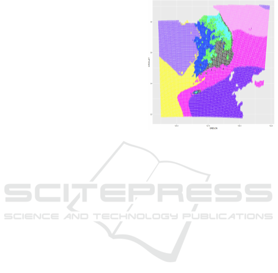
gridded data can be determined. Figure 2 shows an
example of clustering results for gridded data in
South Korea for April.
2.1.2 Cluster Assign for Meteorological Sites
The clustering of meteorological observation stations
is based on the results of cluster analysis of gridded
Figure 2: Clustering result for April temperatures using
gridded data on South Korea.
data. The grid points are clustered with temperature
characters. The observation stations are clustered
such that they are assigned to the cluster to which the
nearest grid points belonged. The distance between
the grid point and station is calculated as the
minimum distance using latitude and longitude.
This grouping method of observation stations can
allocate clusters easily if the location information of
the stations exists, even if new observation stations
are placed or the location of the existing stations are
changed.
2.2 Setting of Error Determination
Criteria
The criteria for determining errors in the temperature
data is set using the method of determining abnormal
values in a normal distribution. In the spatial quality
method, we judge the error based on the hourly mean
and standard deviation calculated from the minute
temperature data for stations identified as a cluster.
Using the mean and standard deviation (σ) hourly by
cluster, the value in the range below (1) can be
determined as normal or an error.
Mean-k× σ < value < Mean-k× σ (1)
To obtain k with an appropriate error rate, we
conduct a case study on the observation data of the
minute temperature from 2013 to 2017.
Development of Spatial Quality Control Method for Temperature Observation Data using Cluster Analysis
365
2.2.1 Test Dataset
More than 600 meteorological observation stations of
KMA exist in South Korea; among them, 525 stations
have been observed continuously for more than 10
years. We use those 525 stations for our case study.
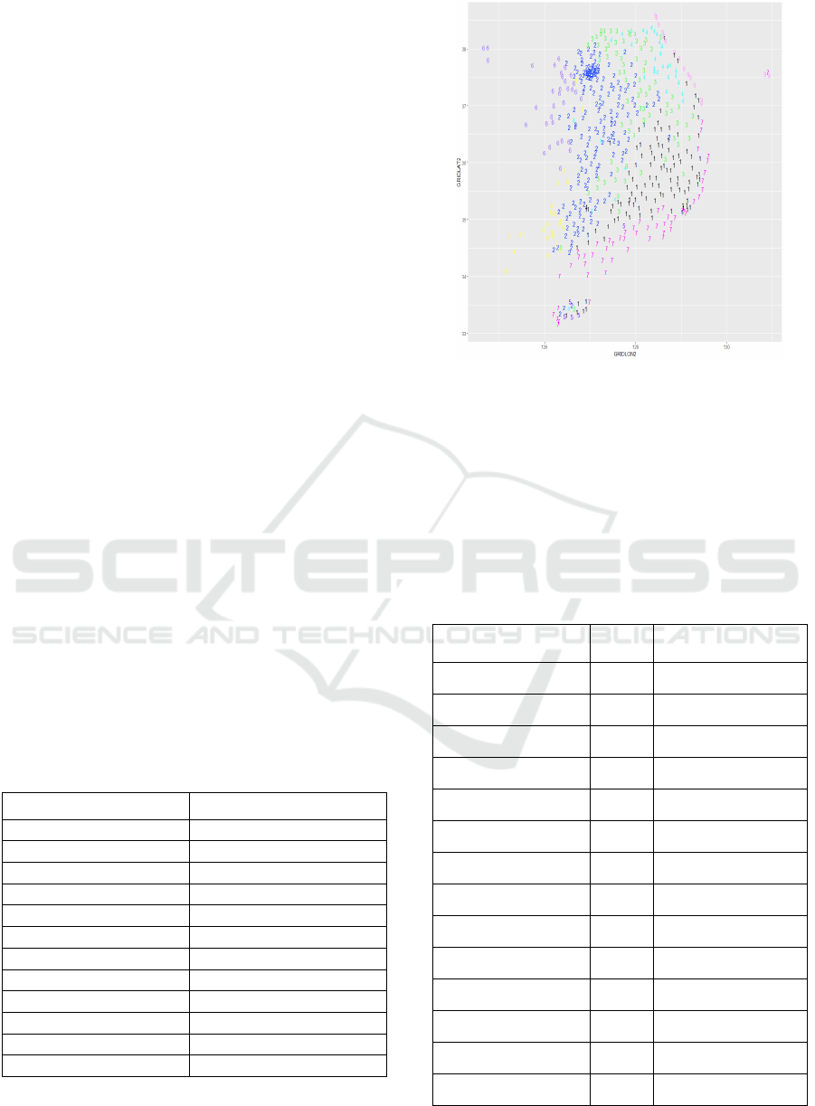
Table 1 shows the number of clusters for the
temperature data of the 525 stations, and Figure 3
shows the example of clustering results for
observation stations in South Korea for April.
The period of data used for the case study is for
2013–2017, and the meteorological parameter is the
temperature observed every minute. Using the result
of clustering, the hourly mean and standard deviation
of the minute temperature for stations classified as a
cluster are calculated.
2.2.2 Test for Setting Error Determination
Criteria
Using the results of the previous calculation, we
confirm whether the values in the standard deviation
interval are normal or errors. Table 2 shows the error
rate by each standard deviation range of every minute
temperature data determined through a case study.
The error rate is calculated as the percentage of the
number of data determined to be errors in the total
data within the range. If the absolute value of the
difference from the mean is less than 7σ, it is
confirmed to be normal; if the absolute value of the
difference is more than 8σ, it is confirmed to be an
error. However, if the absolute value of the difference
is more than 7σ and less than or equal to 8σ, the error
rate is 33.9%, implying that the value in the
distribution range may be normal or an error.
Table 1: Number of clusters by month for meteorological
stations.
Month The number of clusters
January 8
February 7
March 9
April 9
May 10
June 9
July 12
August 10
September 8
October 7
November 7
December 9
Figure 3: Clustering result for temperatures of
meteorological stations in South Korea for April.
In such a case, a manual quality check should be
performed through confirmation of the quality control.
Therefore, in the spatial quality control method,
which is performed automatically, the value is
regarded as an error when the absolute value of
difference from the mean is more than 8σ.
Table 2: Error rate by standard deviation range of every
minute temperature data for 2013–2017.
Range of σ Error rate
Number of data
(error / total)
6σǀrangeǀ7σ
0% 0/6501
7σǀrangeǀ8σ
33.9% 97/286
8σǀrangeǀ9σ
100% 226/226
9σǀrangeǀ10σ
100% 68/68
10σǀrangeǀ11σ
100% 55/55
11σǀrangeǀ12σ
100% 27/27
12σǀrangeǀ13σ
100% 48/48
13σǀrangeǀ14σ
100% 52/52
14σǀrangeǀ15σ
100% 62/62
15σǀrangeǀ16σ
100% 13/13
16σǀrangeǀ17σ
100% 7/7
17σǀrangeǀ18σ
100% 11/11
18σǀrangeǀ19σ
100% 2/2
19σǀrangeǀ20σ
100% 4/4
DATA 2019 - 8th International Conference on Data Science, Technology and Applications
366
3 QUALITY CONTROL RESULTS
3.1 Result of Quality Improvement
We confirm the data quality improvement by
applying the spatial checking method with the criteria
for determining errors derived from the case study.
We apply the spatial method to every-minute
temperature observations for 595 meteorological
observation stations from January 2006 to November
2018. As the period of the numerical model data used
for cluster analysis is from 2006, it is applied to the
data after 2006. By applying the test, 5,915 values
that have been judged normal in the existing methods
are treated as errors. Examples of error handling
through the spatial methods are as follows.
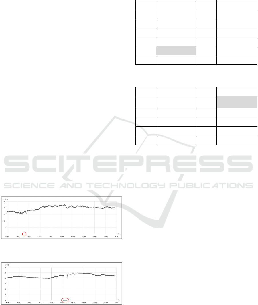
Figure 4 shows the every-minute temperature
distribution at a station in Gageo Island, on June 3,
2016, and the circle is the error-determined part
through the spatial method. Table 3 shows the
temperature data of an error-determined time zone
and the shaded part is the value of the error. The value
of 3:47 is null because it has been refined through the
step check as the variation with the previous value is
more than 3 °C. However, the value of 3:48 has been
determined as normal because the previous value is
refined as an error and no object is available to
calculate the variation, and it is a weak point of the
step check. The spatial method treats that value as an
error, and it is evident that spatial checking can
complement the vulnerable point of the step checking.
Figure 4: Temperature distribution in a station in Gageo
Island, South Korea on June 3, 2016.
Figure 5: Temperature distribution in a station in Yeosu
airport, South Korea on August 29, 2014.
Table 3: Temperature distribution in station in Gageo Island,
South Korea on June 3, 2016.
Time
Temperature(
°C)
Time
Temperature(
°C)
3:44 17.1 3:50 17.2
3:45 17.1 3:51 17.2
3:46 17.1 3:52 17.1
3:47 (null) 3:53 17.1
3:48 0 3:54 16.9
3:49 17.3 3:55 16.9
Table 4: Temperature distribution in a station in Yeosu
airport, South Korea on August 29, 2014.
Time
Temperature(
°C)
Time
Temperature(
°C)
12:11 22.
12:16
~13:05
0
12:12 22. 13:06 (null)
12:13 22. 13:07 20.4
12:14 22. 13:08 21.2
12:15 (null) 13:09 21.9
Figure 5 shows the every-minute temperature
distribution at a station in Yeosu airport, on August
29, 2014, and the circle is the error-determined part
through the spatial method. Table 4 shows the
temperature values of the error-determined time zone,
and the shaded parts of 12:16–13:05 are the values of
errors. The values of 12:16–13:05 have not been
refined through the consistency checking because the
duration of 0 fluctuation is less than 180 min. The
spatial method treats those values as errors; as shown
the spatial checking can complement the vulnerable
point of the time consistency checking.
3.2 Result of Application To Be
Performed Automatically
We apply the spatial checking method to be
performed automatically once daily for data received
later than one day after the observation time. We
measure the time to perform the spatial check of
temperature data in minutes from 595 stations for one
day. The test is performed thrice, and the performance
times are 93 seconds, 59 seconds, and 64 seconds.
The average of performance time is 72 seconds, and
it is considered appropriate to apply the spatial check
automatically to the observation data in minutes.
Development of Spatial Quality Control Method for Temperature Observation Data using Cluster Analysis
367

4 CONCLUSIONS
We develop a new spatial data quality control method
to find errors of temperature observation data based
on clustering for meteorological observation stations.
The threshold of the single station checking method
is the same for all sites; however, the spatial checking
method comprise a segmented threshold spatially and
temporally. Existing spatial tests are time consuming
points to be compared by calculation must be
obtained every time; however, the new spatial test
developed in this study can be performed quickly
because the cluster is set based on the similar climate
characteristics for comparison in advance. Another
advantage is that the spatial checking method can find
errors that have not been found by the methods used
previously. When the observation value of one point
is examined, it cannot be found; however, it is
effective to find an erroneous value that indicated a
large deviation compared with the surrounding points.
High-quality observation data management and
service are anticipated by applying the spatial quality
control method.
REFERENCES
Barnes, S. L., 1964. A technique for maximizing details in
numerical weather map analysis. Journal of Applied
Meteorology, 3(4), 396-409.
Cressman, G. P., 1959. An operational objective analysis
system. Mon. Wea. Rev, 87(10), 367-374.
Dillon, W. R., & Goldstein, M. 1984. Multivariate analysis
methods and applications (No. 519.535 D5).
Kim, H., Kim, K., Lee J., Lee, Y., 2017. Cluster analysis by
month for meteorological stations using a gridded data
for numerical model with temperatures and
precipitation, Journal of the Korean Data &
Information Science Society 2017, 28(5), 1133-1144.
Kim, H., Oh, S., Lee, Y. 2013. Design of heavy rain
advisory decision model based on optimized RBFNNs
using KLAPS reanalysis data. Journal of Korean
Institute of Intelligent Systems, 23(5), 473-478.
Kim, M., Han, M., Jang, D., Baek, S., Lee, W., Kim, Y.,
2012. Production Technique of Observation Grid Data
of 1km Resolution, Climate research, 7(1), 55-68.
Mirkin, B. 2005. Clustering for data mining: a data
recovery approach. Chapman and Hall/CRC.
Murtagh, F. and Legendre, P. 2014. Ward’s hierarchical
agglomerative clustering method: which algorithms
implement Ward’s criterion?. Journal of classification,
31(3), 274-295.
Wagstaff, K., Cardie, C., Rogers, S., Schrődl, S. 2001.
June). Constrained k-means clustering with
background knowledge. In Icml (Vol. 1). 577-584.
Ward Jr, J. H. 1963. Hierarchical grouping to optimize an
objective function. Journal of the American statistical
association, 58(301), 236-244.
WMO. 2013. Guide to the Global Observing System,
WMO-No.488.
DATA 2019 - 8th International Conference on Data Science, Technology and Applications
368
