State Observability through Prior Knowledge:

A Conceptional Paradigm in Inertial Sensing

Tom L. Koller

, Tim Laue

and Udo Frese

Multi-Sensoric Systems, University of Bremen, Enrique-Schmidt-Str. 5, Bremen, Germany

Keywords:

State Estimation, Kalman Filter, Prior Knowledge, Inertial Navigation System (INS), State Observability.

Abstract:

Inertial Navigation Systems suffer from unbounded errors on the position and orientation estimate. Extero-

ceptive sensors may not always be available to correct the error. Applications in the literature overcome this

problem by fusing IMU data with prior knowledge in an ad-hoc fashion. In different applications, various

knowledge is available, which allows to correct the erroneous state estimate. In this position paper, we argue

that the fusion of knowledge and inertial sensor data should be viewed as a paradigm and that the observability

of systems with prior knowledge should be analysed theoretically. With a theoretical foundation, application

design will be simpliﬁed and veriﬁable. We show methods to start the analysis and give a ﬁrst proof with

practical insight.

1 INTRODUCTION

Inertial Navigation Systems (INS) perform dead reck-

oning on the measurements of Inertial Measurement

Units (IMU). This way, the state of an object, consist-

ing of position, orientation and velocity, is estimated.

Dead reckoning has the major disadvantage that the

estimate’s error increases over time. This drift, e.g. a

position error of 1.5 m after only 5 s of dead reckon-

ing (Wenk, 2017, Figure 3.7), is caused by accumu-

lating the measurement errors of the IMU. To correct

the drift, IMU measurements are often fused with ex-

teroceptive position sensors, for example the GPS.

Given this drift, it seems necessary to have an ex-

teroceptive sensor. However, in fact drift-free esti-

mates can be obtained from IMU measurements alone

if appropriate scenario knowledge is exploited. This

surprising realisation motivates our position paper.

There already exist several works that success-

fully demonstrate the usefulness of prior knowledge

in state estimation. The pose (position and orienta-

tion) of humans walking in buildings can be tracked

using prior knowledge instead of exteroceptive sen-

sors (Harle, 2013; Beauregard et al., 2008; Woodman

and Harle, 2008). The estimate errors of the pose are

bounded, which means that the estimates are drift-

https://orcid.org/0000-0001-6629-1566

https://orcid.org/0000-0002-2845-1300

https://orcid.org/0000-0001-8325-6324

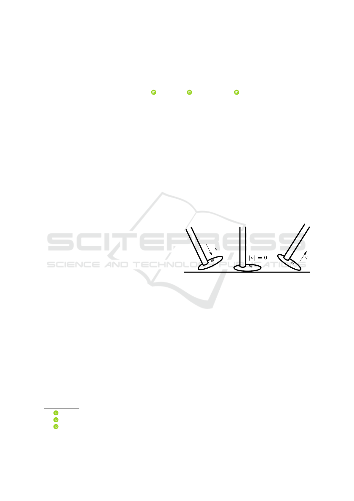
Figure 1: The foot has 0 velocity when it stands on ground.

free. Intuitively, we deﬁne that as observability, and

we will further refer to states that can be estimated

with bounded errors as observable.

The indoor tracking works achieve state observ-

ability through prior knowledge about human motion.

While walking, the feet periodically touch the ground,

wherefore they have 0 velocity at one moment (see

Fig 1). Updating the velocity with this information is

called a Zero-Velocity-Update (ZUPT) and makes the

velocity observable (Foxlin, 2005).

The ZUPTs are used to estimate step lengths,

which are fed to a Particle Filter (PF) as the dynamic

update. The PF models the knowledge that humans

can not pass through walls by removing particles that

cross walls. The used prior knowledge makes the

pose observable and even enables localization with-

out knowing the starting pose (Woodman and Harle,

2008). More surprisingly, the use of the prior knowl-

edge enables to map buildings, using an IMU as the

only sensor (Angermann and Robertson, 2012).

Koller, T., Laue, T. and Frese, U.

State Observability through Prior Knowledge: A Conceptional Paradigm in Inertial Sensing.

DOI: 10.5220/0007952307810788

In Proceedings of the 16th International Conference on Informatics in Control, Automation and Robotics (ICINCO 2019), pages 781-788

ISBN: 978-989-758-380-3

781

Several other works achieve state observability by

combining IMU data with knowledge. Dissanayake

et al. (2001) uses the knowledge, that a wheeled vehi-

cle only moves in forward direction. It is shown that

velocity and inclination are observable if the vehicle

drives a curve. In attitude estimation, several works

use the gravity vector to observe roll and pitch (Va-

ganay et al., 1993; Rehbinder and Hu, 2004; Sabatini,

2006). Wenk (2017, Sec. 3.9) shows that this is equiv-

alent to the prior that the acceleration is 0 in average.

The motion suit of Xsens fuses the measurements of

17 IMUs with the knowledge that they are linked

by the human body joints (Roetenberg et al., 2009).

This enables to observe the angles of all body joints

even without a magnetometer (Wenk, 2017, Sec. 4.4).

Applications with exteroceptive sensors incorporate

knowledge to improve the observability of the state

opez-Araquistain et al., 2019; Xu et al., 2016; Bat-

tistello et al., 2012).

In most cases, the improvement of the estimate

is shown empirically. Instead, the state observability

can be analysed from a theoretical point of view. The

theoretical analysis has the advantage that it reveals

whether the knowledge reduces the state drift or elim-

inates it. This difference is critical, since a reduced

drift still causes an error on long term measurements.

It can be investigated which knowledge makes

which state observable. This may give further insight

about its use and beneﬁts. More importantly, error

cases may be revealed before an application is tested.

The use of prior knowledge is highly beneﬁcial,

but only understood on a per-case basis. It is mainly

evaluated application speciﬁc. Therefore, it misses

theoretical foundation for general applications. So

we argue that fusing prior knowledge with IMU data

should be viewed as a conceptional paradigm and in-

vestigated from a theoretical point of view.

The remainder of the paper is structured as fol-

lows. In Section 2, we explain the gain from under-

standing the paradigm of state observability through

prior knowledge. We will show the structure of prior

knowledge and algorithms to use it. In Section 3, we

will show a method to analyse state observability. We

give an example of its usage in form of a ﬁrst proof

and show how to design an application in track cy-

cling based on the paradigm. At last, we state the

major research goals of our project in Section 4.

2 EXPLAINING THE NEED FOR

A PARADIGM

In application design regarding sensor fusion, we

want to know whether we can estimate the states we

require. The estimate error of unobservable states

increases over time, whereas the error of observable

states is bounded. Hence, we want to achieve observ-

ability of relevant states.

2.1 State Observability

Position:“If we understand the state observability

through prior knowledge, we can predict the error be-

haviour of the estimate.”

For many applications, prior knowledge that may

lead to observability of the relevant states is avail-

able. State observability analysis reveals whether the

knowledge is sufﬁcient to observe the state.

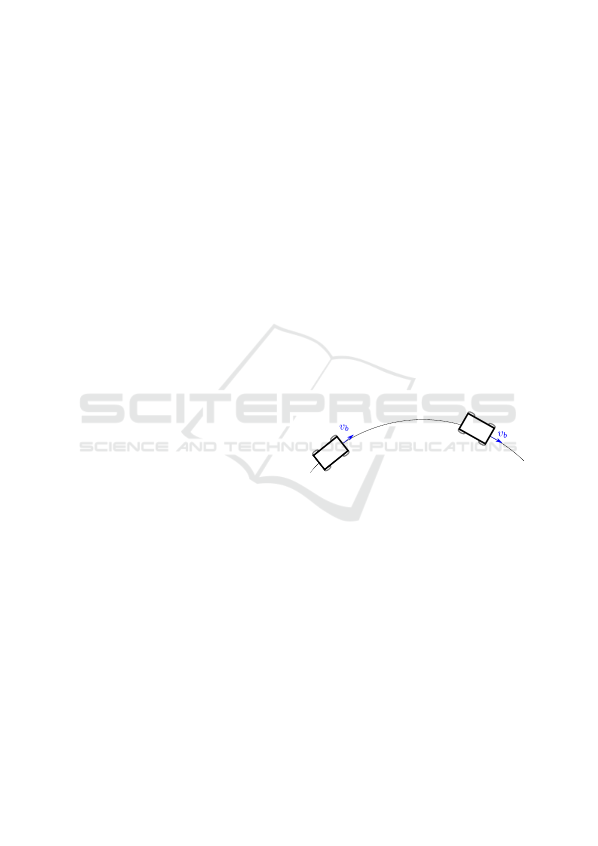
An example of observability analysis can be seen

in (Dissanayake et al., 2001). They use the forward

velocity prior (see Figure 2). It states that the wheeled

vehicle only drives forward with no side slip. This can

be modelled by:



|~v

| 0 0



(1)

where ~v

is the velocity in body coordinates and ~v

the velocity in world coordinates. Whenever the vehi-

cle drives a curve around the y or z axis, the forward

velocity is observable. Additionally, the sensor biases

are observable (Rothman et al., 2014).

Figure 2: Forward velocity prior on a wheeled vehicle.

The collected insight enables us to predict the er-

ror behaviour, instead of measuring it. We can predict

that the velocity error is low while driving curves and

high otherwise. The observations of (Dissanayake

et al., 2001) match this prediction.

As shown, the analysis allows to predict the error

behaviour of the state estimate. Hence, we could vali-

date the quality of the state estimate before we test it.

Therefore, we need the analysis of state observability

through prior knowledge.

Position:“Predicting the error behaviour of a state es-

timator is a powerful tool, which points out knowl-

edge that yields state observability.”

The effect of prior knowledge is dependent on the

state conﬁguration. For example, the forward velocity

prior yields observability of the velocity for a vehicle

driving on a curved line (see Figure 2), but not on a

straight line (see Figure 3). Hence, fusing IMU data

with prior knowledge may not yield state observabil-

ity in all state conﬁgurations.

ICINCO 2019 - 16th International Conference on Informatics in Control, Automation and Robotics

782

Figure 3: Vehcile driving a straight line. The velocity is not

observable with the forward velocity prior.

The observability analysis reveals the observable

and unobservable state space conﬁgurations. A do-

main expert can evaluate how likely the unobservable

conﬁgurations occur. The unobservable conﬁgura-

tions may be isolated points in the state space, which

are surrounded by observable conﬁgurations. Con-

sider a smooth transition between a left and a right

curve. The transition point itself is straight, wherefore

the velocity is unobservable with the forward velocity

prior. However, the velocity can be dead reckoned at

that single point. The accumulated error is negligible.

If the vehicle drives on a straight line during the

whole application, the velocity is unobservable. In

other words, the application takes place in unobserv-

able conﬁgurations only. This is the other extreme,

which makes the prior knowledge useless.

When we evaluate how likely unobservable con-

ﬁgurations occur in the application, we use additional

prior knowledge about the application. The evalu-

ation reveals which additional prior renders the un-

observable conﬁgurations impossible. This prior ei-

ther has to be modelled explicitly, or already makes

the state observable implicitly. In both cases, the ob-

servability analysis points out which assumptions are

needed for state observability.

Overall, the analysis of the observability shows,

whether the application can work. Hence, it can be

used for veriﬁcation of the system design. This is the

most important part of the paradigm of state observ-

ability through prior knowledge. We have to under-

stand how using knowledge corrects the drift or only

improves the state estimate and when it is useless or

even disruptive. In the end, the better the knowledge

is understood, the greater the beneﬁt is.

2.2 Types of Knowledge

Position:“Prior knowledge is structured in several

groups with different observability characteristics.”

In the literature, we ﬁnd various types of prior knowl-

edge. Different knowledge constrains different states

of the state vector. Building plans (Beauregard et al.,

2008), vessel routes (Battistello et al., 2012), ﬂight

corridors (Xu et al., 2016) and road maps (L

opez-

Araquistain et al., 2019) constrain the position of the

object. ZUPTs (Foxlin, 2005) and the forward veloc-

ity prior (Dissanayake et al., 2001) constrain the ve-

locity. The low acceleration prior (Wenk, 2017) con-

Figure 4: Upper and lower y-position bounds (red). Left is

almost an equality constraint. Right has a minor effect.

strains the acceleration.

In many cases, the knowledge can be modelled as

equality or inequality constraint. Equality constraints

reduce the dimension of the state space and occur

if the state is overparametrized. An example is the

quaternion parametrization of rotations. It uses four

states that are constrained to have norm one, instead

of the three rotation angles.

Inequality constraints reduce the state space, but

not its dimension. They often occur in the form of up-

per or lower bounds on a state. Building maps, as they

are used in PFs (Harle, 2013), are a representation of

complex inequality constraints. They model that the

object’s position does not equal the position of a wall.

Particles that violate the constraint are deleted.

In contrast to equality constraints, inequality con-

straints can have different strength (see Figure 4). The

strength of the constraint affects the observability of

the state. Close bounds are almost an equality con-

straint. However, if the bounds are far apart from each

other, the constraint has a minor effect.

In general, constraints are modelled imperfectly.

They are either simpliﬁed or known inexactly. The

imperfection can be grouped into inaccuracy, incom-

pleteness or inconsistency (Podt et al., 2014). An im-

perfect constraint can be modelled as a probability

distribution. However, constraints are often assumed

to model the reality perfectly.

The imperfection of a constraint affects the obser-

vability of the system. Consider the perfect constraint

˙x = 0. x stays at its starting value and is observable.

A similar imperfect constraint ˙x = N (0,σ

) allows

accumulating changes of the state. Hence, it does not

yield observability.

Position:“The structure of prior knowledge may be

exploited to proof observability for general systems.”

Knowledge may be grouped by the type of constraint

it imposes on the system. This allows to investigate

the state observability in a general fashion. Differ-

ent equality constraints reduce the dimension of the

state space in a similar manner. Hence, the observ-

ability can be investigated for general state space de-

scriptions, such as 2D- or 3D-systems.

State Observability through Prior Knowledge: A Conceptional Paradigm in Inertial Sensing

783

In the case of INS, the dynamic equations make

the observability of the states dependent. If the po-

sition is observable, the velocity can be derived by

differentiation. There may be other observability re-

lations between the states.

A general view on the types of knowledge enables

a fast observability analysis without proofs for appli-

cations. With rules and proofs for general systems and

types of knowledge, only the structure of the available

knowledge has to be determined. The observability

characteristics can be derived intuitively by analysing

the observability for each knowledge followed by de-

riving the implied observability. This allows to use

concepts based on the paradigm of state observability

through prior knowledge without prooﬁng the observ-

ability mathematically.

Position:“Structural similarities in prior knowledge

may reveal new possible applications.”

Many assumptions can be transferred on other appli-

cations. For example, the forward velocity prior for

vehicles is valid for bikers as well. If observability

of a prior knowledge has been proofed for one appli-

cation, other suitable applications are likely to exist.

The observability proof can be generalized for simi-

lar applications. Hence, the discovery of a prior that

yields observability reveals that similar applications

are possible, which were previously thought to be im-

possible.

2.3 Algorithms for Prior Knowledge

Position:“A better comprehension of the structure of

prior knowledge may enable new algorithms.”

Using constraints algorithmically in state estimation

is already a topic of research and reviewed in (Simon,

2010; Rasool, 2018). Several methods project either

the state estimate, the Kalman gain or the whole sys-

tem on a constrained subspace. On the subspace, the

constraint is guaranteed to hold.

A common approach is the use of constraints as

pseudo measurements (Tahk and Speyer, 1990). The

constraint is handled as a measurement with a con-

stant measurement observation. This allows an easy

integration in all variants of Kalman ﬁlters. The ap-

proach can be used with perfect and imperfect con-

straints.

In principle, the algorithms search the most proba-

ble solution. This can be formulated as a least squares

minimization problem. The Moving Horizon Estima-

tor solves the least squares problem for a moving win-

dow on the measurements. It can deal with highly

non-linear systems and constraints.

The algorithms solve the state estimation problem

for different assumptions about the system description

and constraints. The performance of each algorithm

depends on the (non-)linearity of the system and the

constraints, and the type of the constraints. Simon

(2010) proposes a decision chart to choose the algo-

rithm based on these parameters. If we understand

the structure of prior knowledge in greater detail, we

can evaluate the algorithm’s performance with regard

to other parameters. Hence, we may choose a better

algorithm or develop a new one that exploits the pe-

culiarities of the knowledge.

3 OBSERVABILITY ANALYSIS

OF PRIOR KNOWLEDGE

In the Introduction, we deﬁned an observable state as

a state that can be estimated with bounded errors. The

estimate of an observable state, does not drift away

from the true value. This deﬁnition is relevant for ap-

plications, because we generally need estimates of the

pose that are always close to the object’s real pose.

For theoretical analysis of prior knowledge, we

will make use of the more formal observability deﬁ-

nitions in (Adamy, 2018) and (Kou et al., 1973) taken

from control theory. Both works assume a system def-

inition as follows:

The system has an unknown state x. The deriva-

tive of the state depends on the known input u and can

be calculated by:

˙x = f (x,u) (2)

with the known function f . The system has an mea-

surable output z deﬁned by:

z = h(x) (3)

with the known function h. State, input and output are

vectors with arbitrary dimension.

Adamy (2018) deﬁnes two forms of observability.

The state is strongly observable if it can be derived

from the in- and outputs of one time point, i.e. without

any data from previous or following time points. In

contrast, the state is weakly observable if it can be

derived from the in- and outputs of a time interval. We

will mainly use weak observability, since the strong

one can not be applied on most non-linear systems.

Kou et al. (1973) deﬁnes observability similar to

uniqueness. The state is observable if there is only

one trajectory, which starts at the known start state

= x(t

) and ﬁts the out- and inputs since the time

point t

. Any ambiguity yields the state unobservable.

We will use this deﬁnition to further analyse why a

state is unobservable and to give advice which prior

knowledge would make the state observable.

ICINCO 2019 - 16th International Conference on Informatics in Control, Automation and Robotics

784

The strength of observability can not be expressed

by the notation of observable or unobservable. An-

other notation is shown in (Han and Wang, 2008),

where a Degree of Observability (DoO) is computed

based on the covariance of the state. The continu-

ous DoO takes sensor noise into account. Consider

a wheeled vehicle with the forward velocity prior. If

the gyrometer error is considerably higher than the

rotation axis change of a curve, it dominates the mea-

surement. Hence, a system can be analytically ob-

servable, whereas the real application is not. In that

case, the DoO would show poor observability for the

velocity. It has to be investigated, how the DoO can

be predicted from the system parameters.

The weak observability after (Adamy, 2018) can

be investigated for prior knowledge that can be mod-

elled as an equality constraint. The main approach

is to observe the states by the time derivatives of the

system’s output equation z = h(x). This results in an

observation vector Z(x) of dimension n, where n is

the state’s dimension.

Z(x) =







h(x)







(4)

The state is observable if x can be derived from Z(x),

which is possible when Z is left invertible:

x = Z

−1

(Z(x)) (5)

Z is left invertible at x if its Jacobian is full ranked at

which yields the weak observability criteria:

rank



)



= n (6)

Evaluating the Jacobian at a state conﬁguration x

, re-

sults in a local form of the observability. If the system

has an equal form at multiple conﬁgurations (see Fig-

ure 5), the correct state can not be determined.

Figure 5: A system with repeating slopes. With the weak

observability criteria only, the correct state is unknown.

3.1 ”Rollercoaster” Observability Proof

We show the application of the observability analysis

in a simple theoretical example. We will proof that

a one dimensional system is weakly observable if the

rotation axis changes. The proof is a ﬁrst step towards

observability analysis for complex systems.

Consider a rollercoaster. It can only ride on the

track, which deﬁnes position and orientation. In other

words, its pose x is a function of the variable λ:

x = f (λ) (7)

All derivatives of the pose, such as the cartesian and

angular velocities, depend on λ and its derivatives:

˙x =

λ · f

(λ) (8)

¨x = (

λ)

· f

(λ) +

λ · f

(λ) (9)

λ is the velocity on the track and

λ the acceleration.

Theorem 1: A system which pose x only depends

on the variable λ is weakly observable from gyrome-

ter measurements if the rotation axis of the orientation

is changing.

Proof: We parametrize the orientation q as a quater-

nion. The orientation quaternion only depends on λ.

q = q(λ) (10)

˙q(λ) =

dλ

(11)

dλ

q(λ) ∗ ω(λ) (12)

Where ω(λ) is the angular velocity as a quaternion

with 0 real part

˙q(λ) =

λ ·

q(λ) ∗ ω(λ) (13)

With the gyrometer we measure z =

λω(λ)

z =

λω(λ) = 2q(λ)

−1

∗

q(λ) (14)

(λ) =



dλ



(15)

Now we proof the full rank of the matrix via linear

independency of the columns:

= k

dλ

+ k

(16)

= k

λ · ω

(λ) + k

· ω(λ) (17)

Equation 17 shows that if

λ is 0, the Jacobian is

singular. This is the trivial case, where the object does

not move. In this case, no system can be observed

from the gyrometer. The other case is when ω

(λ) and

ω(λ) are collinear, meaning that the rotation axis does

not change its direction. Hence, the angular velocity

and acceleration rotating around the same axis is the

only non-trivial unobservable case. This only occurs

at state conﬁgurations where there is either no rotation

State Observability through Prior Knowledge: A Conceptional Paradigm in Inertial Sensing

785

or the rotation axis is constant. Therefore, the system

is observable if the rotation axis changes.

The gathered insight supports the intuitive ob-

servability analysis. Observability can be analysed

for the rollercoaster in Figure 6 without any cal-

culations. Between the red lines, the rotation axis

changes, wherefore the segment is observable. The

other segments are unobservable, because the roller-

coaster turns around a constant axis only. One would

expect to observe a transition from a straight part to

a curved part due to the angular velocity change. But

the transition would result in a similar angular rate

signal as starting at 0 velocity on a curve. Thus, it can

not be observed if the velocity can be 0.

Figure 6: Side view (top) and top-down view (bottom) of a

rollercoaster. The dashed red lines mark the segment with

weak observability after Theorem 1.

Theorem 1 reveals local observability conditions

for general 1D systems. Based on this, we assume

that observability analysis can be performed on more

complex general systems. For example, a general-

isation of Theorem 1 for systems of higher dimen-

sion, where the prior knowledge can be modelled as

an equality constraint of the form:

z = f (x, y) (18)

could be applied in sports like track cycling or For-

mula 1. In these sports, the position can be expressed

with two parameters and the orientation with one.

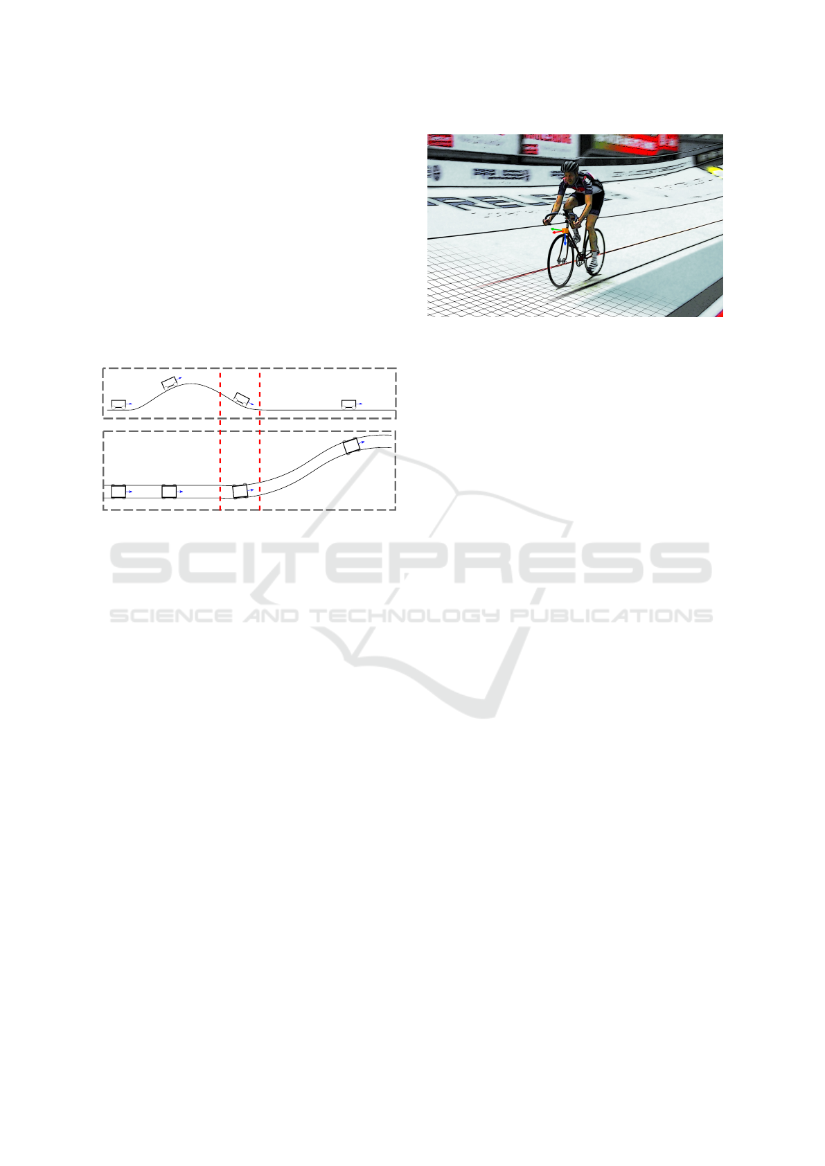
3.2 Track Cycling Design Example

The focus of our research project are theoretical

proofs as in Theorem 1, which give insight about ob-

servability conditions for prior knowledge. Neverthe-

less, we want to show how the gathered insight can

be used in real world scenarios. The forward velocity

prior (Dissanayake et al., 2001) directed us to track

cycling (see Figure 7), which has similar conditions

as the wheeled vehicle. We will argue that the pose

of a track cycler is likely to be observable if available

prior knowledge is fused with IMU data, due to the

track’s shape.

Figure 7: Tracking a biker with an IMU as the only sensor

may be possible with prior knowledge.

At track cycling, bikers run a race on a track. It

is desired to track their velocity and when they drive

in the slipstream of other bikers. To detect whether

a biker drives in the slipstream, the positions of all

bikers are required. The values should be retrieved by

using an IMU at each bike and prior knowledge.

Following the paradigm, we gather knowledge

about the dynamics and constraints of the motion. At

track cycling, both wheels stay on the symmetrical

track. A typical track is shown in Figure 8. The track

is taken counter clockwise. The bikes drive forward

with almost no side slippage, similar to wheeled ve-

hicles. A biker’s speed is limited. Bikers lean into the

curve. We measure the local gravity vector with the

IMU. The starting position of the bikers is known.

With this still incomplete list of knowledge, we try

to analyse the observability of the state. We already

know from (Dissanayake et al., 2001) that the velocity

is observable when we drive a curve with the forward

velocity prior. The bikers follow the track, which con-

tains 2 curves and 2 straight segments. Hence, the

velocity is observable periodically.

Since the wheels of the bike have to be on the

track, the position is constrained and has only 2 DOF.

The height can be calculated from the x and y posi-

tion. We try to use Theorem 1 to make assumptions

about the observability. The theorem states that a 1D

system is observable from gyrometer measurements

alone if the rotation axis changes. At a single round

of track cycling, the biker roughly follows a 1D path

on the track’s 2D surface. In the curves of this path,

the rotation axis changes, which yields observability

after Theorem 1.

At the straight track parts, dead reckoning has to

be performed. In principle, the velocity and position

error will grow unbounded, but only until the biker

drives a curve. Hence, the error growth is practically

bounded, depending on the time the biker drives on

the straight part.

The change of rotation axis can be surely detected,

ICINCO 2019 - 16th International Conference on Informatics in Control, Automation and Robotics

786

Figure 8: The track of the Sixdays Bremen.

but the biker can be in either curve. Thus, if the start-

ing position is unknown, the biker can not be local-

ized uniquely. This ambiguity can be resolved since

the starting position is known. However, the state es-

timator can not recover if it looses the position once.

At long term, roll and pitch are observable due to

the known gravity vector. Since the bikers drive only

counter-clockwise, the yaw can be constrained to fol-

low the path of the track.

The analysis of the state observability shows that

the relevant states, the position and the velocity, can

be expected to have bounded errors if the IMU data is

fused with the knowledge. Therefore, we expect that

the application is possible, which will be evaluated in

a future publication.

The theoretical insight on the prior given by The-

orem 1 and (Dissanayake et al., 2001) revealed the

behaviour of the estimate error. It has to be investi-

gated whether Theorem 1 can be generalized to the

2D case, as it was used in this example, to back up

the approximate argument in this example.

4 CONCLUSION AND FUTURE

WORK

The concept of fusing IMU data with prior knowledge

is already used in the literature. Surprisingly, various

works report bounded errors on normally unobserv-

able states. Their success shows that prior knowledge

has the potential to make states observable. However,

only a few works provide a theoretical foundation for

the observability.

By analysing the observability of states in appli-

cations with prior knowledge, we can predict the er-

ror behaviour of the state estimate. Thus, applications

can be veriﬁed before testing. Possible failure cases

can be predicted from the observability conditions re-

vealed by the analysis.

We have shown suitable methods, taken from the

ﬁeld of control theory, to analyse the state observ-

ability in applications with equality constraints. We

started to investigate the observability conditions for

simple systems. At a ﬁrst shot, we found Theorem 1,

which states that a 1D system is observable if its rota-

tion axis changes. The method can be used to validate

the design of applications before testing it.

Prior knowledge is structured into groups with

different observability characteristics. Analysing the

groups will result in a better comprehension of prior

knowledge. The comprehension can point out appli-

cations that were thought to be impossible with IMUs

alone, such as the tracking of bikers at track cycling.

The utility of prior knowledge depends on the re-

quired estimation accuracy, modelling errors and the

sensor noise. This results in different grades of state

observability through prior knowledge. Theoretical

observability alone, can only guarantee bounded er-

rors for precise models of the real world applications.

It has to be investigated how the utility of prior knowl-

edge can be estimated for imperfect conditions.

The paradigm of state observability through prior

knowledge aims at understanding the inﬂuence of

prior knowledge on the observability of the state es-

timate. With the investigation of the paradigm, we

expect to simplify the analysis of the state observabil-

ity by prooﬁng observability for structural groups of

prior knowledge. The gained theoretical insight will

result in faster application development and enables

veriﬁcation of state estimation systems.

In our research project, we focus on the theoretical

foundation of prior knowledge. We will further anal-

yse general system descriptions, such as 2D systems.

We will derive and investigate common structures in

prior knowledge from existing applications to proof

observability in generalized cases. Our results will be

interpreted from an intuitive point of view. This will

allow a wide audience to use our results without exe-

State Observability through Prior Knowledge: A Conceptional Paradigm in Inertial Sensing

787

cuting the analysis themselves.

The theoretical results will be accompanied by ap-

plication examples from the ﬁeld of sports science.

Since most sports follow a rulebook, various kinds of

prior knowledge can be applied. Player policies can

be used to investigate vague prior knowledge.

ACKNOWLEDGEMENTS

This project (ZaVI FR 2620/3-1) is funded by the

German Research Foundation.

REFERENCES

Adamy, J. (2018). Nichtlineare Systeme und Regelungen.

Springer.

Angermann, M. and Robertson, P. (2012). FootSLAM:

Pedestrian simultaneous localization and mapping

without exteroceptive sensors;hitchhiking on human

perception and cognition. Proceedings of the IEEE,

100(Special Centennial Issue):1840–1848.

Battistello, G., Ulmke, M., Papi, F., Podt, M., and Boers,

Y. (2012). Assessment of vessel route information use

in bayesian non-linear ﬁltering. In 2012 15th Interna-

tional Conference on Information Fusion, pages 447–

454.

Beauregard, S., Widyawan, and Klepal, M. (2008). Indoor

PDR performance enhancement using minimal map

information and particle ﬁlters. In 2008 IEEE/ION

Position, Location and Navigation Symposium, pages

141–147.

Dissanayake, G., Sukkarieh, S., Nebot, E., and Durrant-

Whyte, H. (2001). The aiding of a low-cost strap-

down inertial measurement unit using vehicle model

constraints for land vehicle applications. IEEE trans-

actions on robotics and automation, 17(5):731–747.

Foxlin, E. (2005). Pedestrian tracking with shoe-mounted

inertial sensors. IEEE Computer Graphics and Appli-

cations, 25(6):38–46.

Han, S. and Wang, J. (2008). Monitoring degree of ob-

servability in GPS/INS integration. In International

Symposium on GPS/GNSS.

Harle, R. (2013). A survey of indoor inertial positioning

systems for pedestrians. IEEE Communications Sur-

veys and Tutorials, 15(3):1281–1293.

Kou, S. R., Elliott, D. L., and Tarn, T. J. (1973). Observ-

ability of nonlinear systems. Information and Control,

22(1):89–99.

opez-Araquistain, J.,

Angel J. Jarama, Besada, J. A.,

de Miguel, G., and Casar, J. R. (2019). A new ap-

proach to map-assisted bayesian tracking ﬁltering. In-

formation Fusion, 45:79 – 95.

Podt, M., Bootsveld, M., Boers, Y., and Papi, F. (2014).

Exploiting imprecise constraints in particle ﬁltering

based target tracking. In Information Fusion (FU-

SION), 2014 17th International Conference on, pages

1–8. IEEE.

Rasool, G. (2018). Constrained state estimation-a review.

arXiv preprint arXiv:1807.03463.

Rehbinder, H. and Hu, X. (2004). Drift-free attitude es-

timation for accelerated rigid bodies. Automatica,

40(4):653 – 659.

Roetenberg, D., Luinge, H., and Slycke, P. (2009). Xsens

MVN: Full 6DOF human motion tracking using

miniature inertial sensors. Xsens Motion Technol. BV

Tech. Rep., 3.

Rothman, Y., Klein, I., and Filin, S. (2014). Analytical ob-

servability analysis of INS with vehicle constraints.

Navigation: Journal of The Institute of Navigation,

61(3):227–236.

Sabatini, A. M. (2006). Quaternion-based extended kalman

ﬁlter for determining orientation by inertial and mag-

netic sensing. IEEE Transactions on Biomedical En-

gineering, 53(7):1346–1356.

Simon, D. (2010). Kalman ﬁltering with state constraints: a

survey of linear and nonlinear algorithms. IET Control

Theory & Applications, 4(8):1303–1318.

Tahk, M. and Speyer, J. L. (1990). Target tracking problems

subject to kinematic constraints. IEEE transactions on

automatic control, 35(3):324–326.

Vaganay, J., Aldon, M. J., and Fournier, A. (1993). Mobile

robot attitude estimation by fusion of inertial data. In

[1993] Proceedings IEEE International Conference

on Robotics and Automation, pages 277–282 vol.1.

Wenk, F. (2017). Inertial Motion Capturing Rigid Body

Pose and Posture Estimation with Inertial Sensors.

PhD thesis, University of Bremen.

Woodman, O. and Harle, R. (2008). Pedestrian localisation

for indoor environments. In Proceedings of the 10th

International Conference on Ubiquitous Computing,

UbiComp ’08, pages 114–123, New York, NY, USA.

ACM.

Xu, L., Liang, Y., Pan, Q., Duan, Z., and Zhou, G. (2016).

A kinematic model of route-based target tracking: Di-

rect discrete-time form. In 2016 19th International

Conference on Information Fusion (FUSION), pages

225–231.

ICINCO 2019 - 16th International Conference on Informatics in Control, Automation and Robotics

788