Point-cloud Mapping using Lidar Mounted on
Two-wheeled Vehicle based on NDT Scan Matching
Kohei Tokorodani
1
, Masafumi Hashimoto
2a
, Yusuke Aihara
1
and Kazuhiko Takahashi
2
1
Graduate School of Doshisha University, Kyotanabe, Kyoto 6100321, Japan
2
Faculty of Science and Engineering, Doshisha University, Kyotanabe, Kyoto 6100321, Japan
Keywords: Two-wheeled Vehicle, Lidar, Point-cloud Mapping, NDT Scan Matching, Distortion Correction, Extended
Kalman Filter, Interpolation.
Abstract: This paper presents a method for generating a 3D point-cloud map using multilayer lidar mounted on two-
wheeled vehicle. The vehicle identifies its own 3D pose (position and attitude angle) in a lidar-scan period
using the normal distributions transform (NDT) scan-matching method. The vehicle’s pose is updated in a
period shorter than the lidar-scan period using its attitude angle and angular velocity measured by an inertial
measurement unit (IMU). The pose estimation is based on the extended Kalman filter (EKF) under the
assumption that the vehicle moves at nearly constant translational and angular velocities. The vehicle’s pose
is further estimated in a period shorter than measurement period of the IMU using a linear interpolation
method. The estimated poses of the vehicle are applied to distortion correction of lidar-scan data, and a point-
cloud map is generated based on the corrected lidar-scan data. Experimental results of mapping a road
environment using a 32-layer lidar mounted on a bicycle show the efficancy of the proposed method in
comparison with conventional methods of distortion correction of lidar-scan data.
1 INTRODUCTION
In recent years, many studies have been conducted on
the active safety and autonomous driving of vehicles
and personal mobility devices. There are also many
studies on last mile automation by delivery robots.
Important technologies in these studies include the
environmental map generation (Cadena et al., 2016)
and map-matching based self-pose estimation by
vehicles using the generated environment maps
(Wang, et al., 2017).
In this study, we focus on map generation with a
lidar mounted on a vehicle. In intelligent
transportation systems (ITS) domains, maps are being
generated using mobile mapping systems (Seif and
Hu, 2016). Their maps are applied to autonomous
driving and active safety for automobiles in wide road
environments, such as highways, and major arterial
roads. In this study, we consider environment maps
for active safety and autonomous driving of personal
mobility devices and delivery robots as well as for
various social services such as disaster prevention and
a
https://orcid.org/0000-0003-2274-2366
mitigation (Schwesinger et al., 2017, Morita et al.,
2019).
To that end, we generate 3D point-cloud maps in
narrow road environments, such as community roads
and scenic roads in urban and mountainous areas,
using lidar mounted on two-wheeled vehicles
(bicycles and motorcycles) with higher
maneuverability than four-wheeled vehicles. To
generate 3D point-cloud maps using an onboard lidar,
lidar-scan data captured in the sensor coordinate
frame have to be accurately mapped on the world
coordinate frame using pose (i.e., position and
attitude angle) information of the vehicle. Since the
lidar obtains scan data by laser scanning, all scan data
within one scan cannot be obtained at the same time
when a vehicle is moving or is changing its attitude.
Therefore, if all scan data within one scan are
transformed based on the vehicle’s pose at the same
time, distortion occurs in scan data mapped on the
world coordinate frame.
To reduce distortion in the scan data, several
methods have been proposed (Brenneke et al., 2003,
Hong et al., 2010, Kawahara et al., 2006, Moosmann
446
Tokorodani, K., Hashimoto, M., Aihara, Y. and Takahashi, K.
Point-cloud Mapping using Lidar Mounted on Two-wheeled Vehicle based on NDT Scan Matching.
DOI: 10.5220/0007946204460452
In Proceedings of the 16th International Conference on Informatics in Control, Automation and Robotics (ICINCO 2019), pages 446-452
ISBN: 978-989-758-380-3
Copyright
c
 2019 by SCITEPRESS – Science and Technology Publications, Lda. All rights reserved

and Stiller, 2011, Zhang and Singh, 2014), in which
the information of global navigation satellite system
(GNSS), inertial measurement unit (IMU), or wheel
encoder is observed within a short period, and the
vehicle’s pose is estimated in a period shorter than the
lidar-scan period. In urban and mountainous
environments, the GNSS information is often denied.
Therefore, for the application in GNSS-denied
environments, we proposed a method to correct
distortion in the scan data using the normal
distributions transform (NDT) scan matching and the
extended Kalman filter (EKF) using only lidar
information (Inui et al., 2017).
Most conventional methods were intended to
correct distortion in lidar-scan data from a lidar
mounted on four-wheeled vehicles, such as
automobiles and mobile robots, moving on flat road
surfaces. To the best of our knowledge, studies that
have handled distortion correction when vehicles
change their poses drastically are very few. Although
several studies (Bosse et al., 2012, Kuramachi et al.,
2015, Zhang and Singh, 2014) handled distortion
correction in lidar-scan data from lidars with pose
changes, their lidars were hand-held lidars which
slowly change their poses.
Thus, in this paper, we propose a method that
generates 3D point-cloud maps by correcting
distortion in the scan data obtained from lidars
mounted on two-wheeled vehicles that change their
pose drastically, compared to lidars mounted on four-
wheeled vehicles and hand-held lidars.
The rest of this paper is organized as follows. In
Section 2, we give an overview of the experimental
system. In Section 3, we summarize scan-data
mapping based on the NDT scan matching. In Section
4, we present the distortion correction and mapping
methods. In Section 5, we conduct experiments to
reveal the performance of the proposed method,
followed by conclusions in Section 6.
2 EXPERIMENTAL SYSTEM
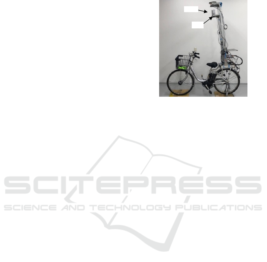
Figure 1 shows the overview of the two-wheeled
vehicle (YAMAHA electric bicycle). As the first step
of the study, we use the bicycle as a two-wheeled
vehicle.
On the upper part of the bicycle, a 32-layer lidar
(Velodyne HDL-32E) and IMU (Tokyo Aircraft
Instrument CSM-MG200) are mounted. The
maximum range of the lidar is 70 m, the horizontal
viewing angle is 360° with a resolution of 0.16°, and
the vertical viewing angle is 41.34° with a resolution
of 1.33°. The lidar provides 384 measurements (the
Figure 1: Overview of experimental bicycle.
object’s 3D position and reflection intensity) every
0.55 ms (at 2° horizontal angle increments). The
period for the lidar beam to complete one rotation
(360°) in the horizontal direction is 100 ms, and
70,000 measurements are obtained in one rotation.
The IMU outputs attitude angles (roll and pitch
angles) and their angular velocities every 10 ms. The
resolution of attitude angle is 6.0×10
-3
° and its error
is ±0.5° (typ.). The resolution of angular velocity is
0.03 °/s, and its error is ±0.5 °/s (typ.).
In this paper, one rotation of the lidar beam in the
horizontal direction (360°) is referred to as one scan,
and the data obtained from this scan is referred to as
scan data. The lidar’s scan period (100 ms) is denoted
as

and scan-data observation period (0.55 ms) as


. The observation period (10 ms) of IMU is
denoted as
I
MU


. Therefore, IMU data are obtained
10 times in one scan of the lidar (τ = 10Δτ
IMU
), and
lidar-scan data are obtained 18 times within the
observation period of IMU (Δτ
IMU
=18Δτ).
3 SCAN-DATA MAPPING USING
NDT SCAN MATCHING
In the process for scan-data mapping using the NDT
scan matching, the scan data captured in the sensor
coordinate frame is mapped onto a 3D grid map (a
voxel map) represented in the bicycle coordinate
frame
b

. A voxel grid filter (Munaro et al., 2012) is
applied to downsize the scan data. The voxel used for
the voxel grid filter is a cube with a side-length of 0.2
m.
In the world coordinate frame
W

, a voxel map
with a voxel size of 1 m is used for the NDT scan
matching. For the i-th (i = 1, 2, …n) measurement in
Lida
r
IMU
Point-cloud Mapping using Lidar Mounted on Two-wheeled Vehicle based on NDT Scan Matching
447

the scan data, we define the position vector in
b

as
bi
p
and that in
W

as
i
p
. Then, the following
relationship is given:

















1
)(
1
bii
p
XΤ
p
(1)
where
T
zyx ),,,,,(  X
is the bicycle’s pose.
T
zyx ),,(
and
T
),,( 
are the 3D position and
attitude angle (roll, pitch, and yaw angles) of the
bicycle, respectively, in
W

. T(X) is the following
homogeneous transformation matrix:


















1000
coscoscossinsin
cossinsinsincoscoscossinsinsinsincos
sinsincossincossincoscossinsincoscos
)(
z
y
x
Τ



X
The scan data obtained at the current time
 t
(t =
0, 1, 2, …)
,

)()(
2
)(
1
)( ,,, t
bn
t
b
t
b
t
b
pppP 
or
,{ )(
1
)( tt pP 
,, )(
2
 t p } )(t
n
p
, are referred to as the new input scan,
and the scan data obtained in the previous time before
 )1( t
,

)1()1()0( ,,,   t PPPP 
, is referred to as the
reference scan.
The NDT scan matching (Biber and Strasser,
2003) conducts a normal distribution transformation
for the reference scan in each grid on the voxel map;
it calculates the mean and covariance of the 3D
positions of the lidar-scan data. By matching the new
input scan at
 t
with the reference scan obtained
prior to
 )1( t , the bicycle’s pose
)(t X
at
 t
is
determined. The bicycle’s pose is used for conducting
a coordinate transform by Eq. (1), and the new input
scan is then mapped to
W

.
In this study, we use point cloud library (PCL) for
the NDT scan matching (Rusu and Cousin, 2011). It
should be noted that the downsized scan data is only
used to calculate the bicycle’s pose using the NDT
scan matching at small computational cost.
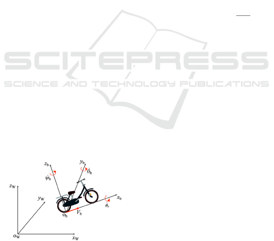
Figure 2: Notation related to bicycle motion.
4 DISTORTION CORRECTION
AND MAPPING
4.1 Motion and Measurement Models
As shown in Fig. 2, the linear velocity of the bicycle
in
b

is denoted as V
b
(the velocity in the x
b
-axis
direction), and the angular velocities about the x
b
-,
y
b
-, and z
b
- axes are denoted as
b


,
b


, and
b


,
respectively.
If the bicycle is assumed to move at nearly
constant linear and angular velocities, the following
motion model can be derived (Inui et al., 2017):


























































































b
b
b
b
w
w
w
wV
aa
aa
aa
az
ay
ax
V
z
y
x
t
b
t
b
t
b
V
t
b
t
ttttt
ttttt
tttttt
ttt
tttt
tttt
t
b
t
b
t
b
t
b
t
t
t
t
t
t






























)(
)(
)(
)(
)(
)()(
3
)()(
2
)(
)()(
3
)()(
2
)(
)()()(
3
)()(
2
)(
)()(
1
)(
)()()(
1
)(
)()()(
1
)(
)1(
)1(
)1(
)1(
)1(
)1(
)1(
)1(
)1(
)
1(
cos
1
cossin
sincos
tancossin
sin
sincos
coscos
(2)
where
2/
2
)()(
1
b
V
t
b
t
wVa

 
,
 )()(
2
t
b
t a


2/
2
b
w




, and
2/
2
)()(
3
b
wa t
b
t





.
b
V
w

,
b
w


,
b
w


, and
b
w


are the acceleration disturbances.
We express Eq. (2) in the following vector form:


 ,, )()1( wξfξ tt  
(3)
where
T
bbbb
Vzyx ),,,,,,,,,( 


ξ
and
w
T
V
b
bb
b
wwww ),,,(




.
The attitude angle and angular velocity of the
bicycle obtained at time
IM U
t 
by IMU is denoted as
()
IMU
tz
. The measurement model is then
() () ()
IMU IMU IMU
ttt  zHξ z
(4)
where
IMU
 z
is sensor noise, and H
IMU
is a
measurement matrix.
We also denote the bicycle’s pose obtained at
 t
using the NDT scan matching as
)()(
ˆ
tt
NDT
Xz 
. The
measurement model is then
() () ()
NDT NDT NDT
ttt  zHξ z
(5)
where
NDT
z 
is the measurement noise, and H
NDT
is
the measurement matrix.
ICINCO 2019 - 16th International Conference on Informatics in Control, Automation and Robotics
448

4.2 Distortion Correction
Figure 3 shows the sequence for correcting distortion
in the lidar-scan data. When at the time
(1) ( 1)
IMU
tk  
, where k =1–10, the state
estimate of the bicycle,
(1)
(1)
ˆ
k
t


ξ
, and its associated
error covariance
(1)
(1)
k
t


Γ
are obtained, the EKF
prediction algorithm (Yaakov et al., 2001) gives the
state prediction
(/ 1)
(1)
ˆ
kk
t


ξ
and its error covariance
(/ 1)
(1)
kk
t


Γ
at the time  )1( t +
IMU
k 
by
(/ 1) ( 1)
(/ 1) ( 1)
ˆ
ˆ
(1) [ (1),0, ]
(1) (1) (1)(1)
( 1) ( 1)
kk k
IMU
kk k T
T
tt
tt tt
tt




 

   


 

ξ f ξ
Γ F Γ F
GQG
(6)
where F =
ξf
ˆ
/
, G = wf  / , and Q is the
covariance matrix of the plant noise, w.
At the time
(1)
IMU
tk  
, we observe the
attitude angle and angular velocity
IMU
z
of the
bicycle with IMU. T
he EKF estimation algorithm
(Yaakov et al., 2001) then gives a state estimate
()
(1)
ˆ
k
t 
ξ
and its error covariance
()
(1)
k
t 
Γ
as
follows:
() (/ 1)
(/ 1)
() (/ 1)
(/ 1)
ˆˆ
(1) (1) {
ˆ
( 1)}
(1) (1)
( 1)
kkk
IMU
kk
IMU
kkk
kk
IMU
tt
t
tt
t





 




 




ξξ Kz
H ξ
ΓΓ
KH Γ
(7)
where
(/ 1) 1
(1) (1)
kk T
tt
IMU


K Γ HS
and
(/ 1)
(1)
kk T
t
IMU IMU IMU


SH Γ HR
. R
IMU
is the
covariance matrix of the sensor noise Δz
IMU
.
We denote the state estimate related to the
bicycle’s pose
),,,,,(  zyx as
() ()
(1) (1)
ˆ
ˆ
kk
tt
X ξ
.
Using the state estimates
(1)
(1)
ˆ
k
t


X
and
()
(1)
ˆ
k
t 
X
at the time
(1) ( 1)
IMU
tk  
and
 )1( t +
IMU
k 
, respectively, the pose
(1)
(1,)
ˆ
k
tj


X
of the bicycle at the time
 )1( t +
(1)
IMU
k  
jΔτ,
where j = 1–17, is interpolated by
(1) (1)
() ( 1)
ˆˆ
(1,) (1)
ˆ
ˆ
(1) (1)
kk
kk
IMU
tj t
tt
j




 
 

XX
XX
(8)
Then, the scan data
(1)
(1,)
k
tj
bi


p
obtained at the
time
 )1( t +
(1)
IMU
k  
jΔτ is transformed to
(1)
(1,)
k
tj
i


p
as follows:
(1) (1)
(1)
( 1,) ( 1,)
ˆ
((1,))
11
kk
k
ibi
tj tj
tj



 


 
 
pp
X
(9)
Figure 3: Sequence of correcting distortion in the scan data.
Using the pose estimate
(10)
(1)
ˆ
t  X
of the bicycle,
the scan data
(1)
(1,)
k
tj
i


p
are again transformed to the
scan data
*
()t
bi
P
in at the time
 t
by
*(1)
(10) 1
() ( 1, )
ˆ
((1))
11
k
bi i
ttj
t



  


  
  
pp
X
(10)
The scan data corrected with Eq. (10),


*** *
() () () ()
12
,,, ttt t
bbb bn
Ppp p
, are used as the new
input scan for scan matching, and the pose angle
NDT
z
of the bicycle at the time
 t
is calculated. In this scan
matching, we use the estimate
(10 )
ˆ
(1)t X
as the
initial pose in the recursive calculation. Then, the
EKF estimation algorithm calculates the state
estimate
()
ˆ
t ξ
and its error covariance
()t Γ
of the
bicycle at the time
 t
as follows:
(10) (10)
(10) (10)
ˆˆ
ˆ
() ( 1) (){ () ( 1)}
() ( 1) () ( 1)
NDT NDT
NDT
tt tt t
ttt t

  


 


ξξ Kz Hξ
ΓΓ KH Γ
(11)
where,
(10 ) 1
() ( 1) ()
T
tt t
NDT


K Γ HS ,
(10 )
() ( 1)
T
tt
NDT NDT NDT

SHΓ HR , and
NDT
R
is
the covariance matrix of .
4.3 Map Generation
We generate the map using the scan data corrected in
the previous section.
When the state estimate
(1)
ˆ
t  ξ
and its error
covariance
(1) t  Γ
of the bicycle are obtained at the
time
 )1( t , the EKF prediction algoritm obtains the
state prediction
(/ 1)
ˆ
tt ξ
and its error covariance
(/ 1) tt  Γ
at the time
t 
as follows:
b

NDT
z

Point-cloud Mapping using Lidar Mounted on Two-wheeled Vehicle based on NDT Scan Matching
449

ˆ
ˆ
(/ 1) [( 1),0,]
( / 1) ( 1) ( 1) ( 1)
( 1) ( 1)
T
T
tt t
tt t t t
tt


 

   


 

ξ f ξ
Γ F Γ F
GQG
(12)
Here, we denote the state prediction related to the
bicycle’s pose
),,,,,(  zyx as
(/ 1) (/ 1)
ˆ
ˆ
tt ttX ξ
.
We use the corrected scan data


*** *
() () () ()
12
,,, ttt t
bbb bn
Ppp p
as the new input scan to
perform scan matching. Then, we calculate the pose
NDT
z
of the bicycle at the time
t 
. In this scan
matching, we use the prediction,
(/ 1)
ˆ
tt X
as the
initial pose in the recursive calculation.
The new input scan
*
()t
b
P
is mapped on the world
coordinate frame
W

using
()
NDT
Tz
in Eq. (1).
Then, the EKF estimation algorithm calculates the
state estimate
()
ˆ
t ξ
and its error covariance
()t Γ
at
the time
 t
as follows:
ˆ
ˆˆ
() ( / 1) (){ () ( / 1)}
() ( / 1) () ( / 1)
NDT NDT
NDT
ttt t t tt
ttt t tt

  


 


ξξ Kz Hξ
ΓΓ KH Γ
(13)
where
1
() ( / 1) ()
T
ttt t
NDT


K Γ HS
and
() ( / 1)
T
ttt
NDT NDT NDT
 SHΓ HR
.
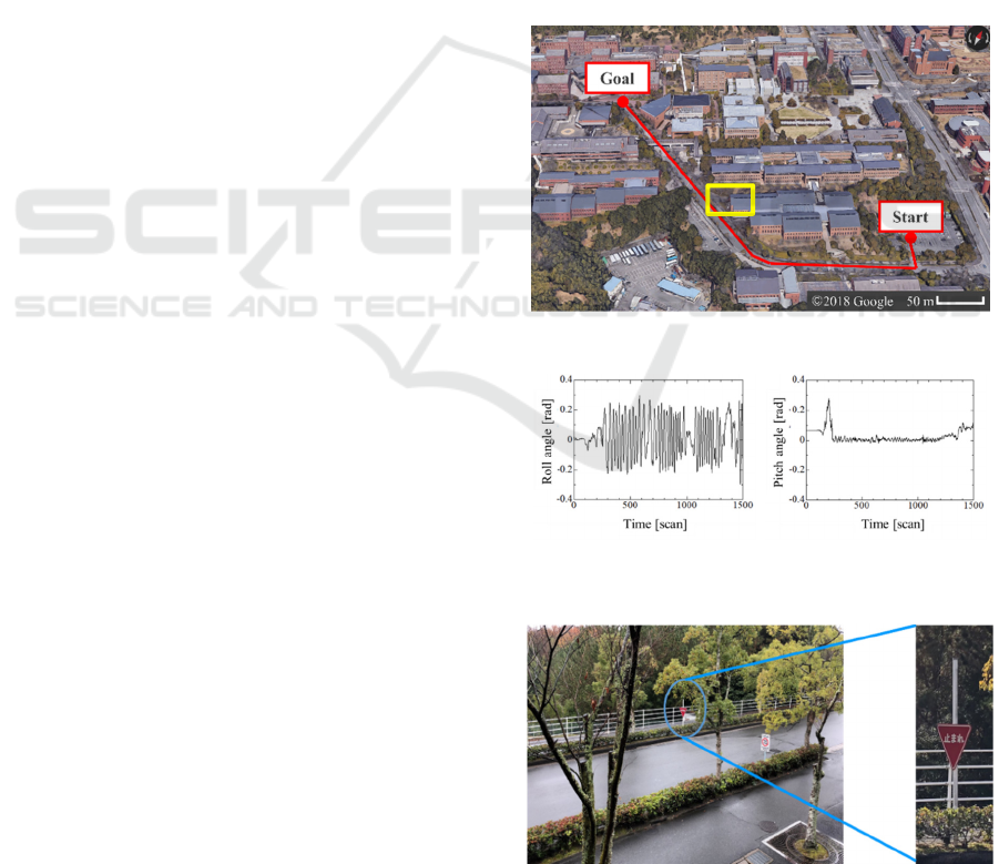
5 EXPERIMENTAL RESULTS
The bicycle moved on a road shown in Fig. 4, and
lidar-scan data in 1500 scans (150 seconds) were
captured. The maximum velocity of the bicycle was
18 km/h. Figure 5 shows IMU output of roll and pitch
angles of the bicycle. To change the attitude of the
lidar largely, the bicycle was moved in zigzag. Then,
the large rolling motions of the bicycle occurred as
shown in Fig. 5 (a).
We evaluate mapping performance in the
following four cases:
Case 1: Mapping by the proposed method
Case 2: Mapping without distortion correction
Case 3: Mapping by our previous method (Inui et.
al., 2017)
Case 4: Mapping using lidar-scan data, in which
distortion is corrected using pose information from
onboard GNSS/ IMU unit
In case 3, we correct distortion in the lidar-scan
data using only the lidar information (using no IMU
information); a bicycle identifies its own 3D pose in
a lidar-scan period (0.1 s) using the NDT scan
matching. Based on the pose information, the
bicycle’s pose is estimated every 0.55 ms using the
EKF, in which Eqs. (3) and (5) are used as motion and
measurement models, respectively. We then
corrected the lidar-scan distortion by the estimated
pose.
The bicycle is equipped with the GNSS/IMU unit
(Novatel, PwrPak7-E1) to evaluate the bicycle
motion in experiments. The root mean square error
(RMSE) in horizontal and vertical positions of the
GNSS/IMU unit are 0.02 m and 0.03 m, respectively.
The RMSE in role/pitch and yaw angles are 0.03° and
0.1°, respectively. In case 4, we measure the bicycle’s
pose every 0.1s with the GNSS/IMU unit and
estimate the bicycle’s pose every 0.55 ms using the
interpolation method. We then correct the lidar-scan
distortion by the interpolated pose.
Figure 6 (a) shows the close-up view of yellow
rectangular area shown in Fig. 4. Figure 7 shows the
mapping result of the environment in Fig. 6 (a).
Figure 8 also shows the mapping result of the traffic
sign in Fig. 6(b) and neighbouring tree.
Figure 4: Experimental environment (bird-eye view).
(a) Roll angle. (b) Pitch angle.
Figure 5: Attitude angle of bicycle.
(a) Mapping environment. (b) Traffic sign.
Figure 6: Mapping environment and traffic sign.
ICINCO 2019 - 16th International Conference on Informatics in Control, Automation and Robotics
450

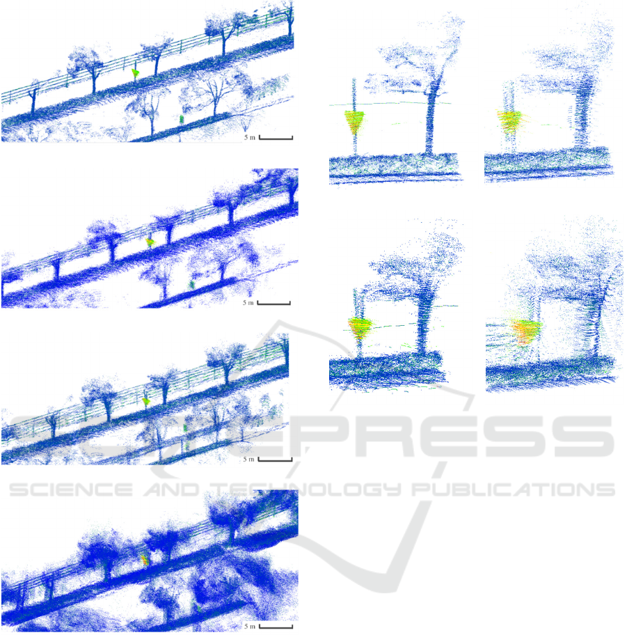
(a) Case 1 (using proposed method).
(b) Case 2 (without distortion correction).
(c) Case 3 (using previous method).
(d) Case 4 (using distortion correction by pose information
from GNSS/IMU unit).
Figure 7: Result of environment mapping. Different
coloured dots indicate lidar-scan data with different
reflective intensities.
It is clear from Figs. 7 and 8 that the mapping
result by the proposed method (case 1) is more
crispness than that by the other methods.
(a) Case 1. (b) Case 2.
(c) Case 3. (d) Case 4.
Figure 8: Mapping result of traffic sign and tree.
6 CONCLUSIONS
In this paper, we proposed a method to generate 3D
point-cloud maps with a lidar mounted on a two-
wheeled vehicle. Distortion in lidar-scan data that
occur by sudden changes of the vehicle’s pose were
corrected; pose of the two-wheeled vehicle were
calculated by the NDT scan matching using the lidar-
scan data obtained at each scan period.
The distortion in the scan data was corrected by
estimating the vehicle’s pose in a period shorter than
the scan period via the EKF and interpolation method
using the information of the NDT scan matching and
IMU. The corrected scan data were applied to
accurate 3D point-cloud mapping.
The experimental results of road-environment
mapping by a 32-layer lidar mounted on a bicycle
validated the efficacy of the proposed method.
As future works, we will perform reduction in
computational costs in mapping, quantitative
evaluation of the mapping performance, and
experiments using a lidar mounted on a motorcycle.
Point-cloud Mapping using Lidar Mounted on Two-wheeled Vehicle based on NDT Scan Matching
451

ACKNOWLEDGEMENTS
This study was partially supported by the JSPS- Japan
Society for the Promotion of Science (Scientific
Grants, Foundation Research (C) No.18K04062).
REFERENCES
Biber, P., and Strasser, W., 2003, The Normal Distributions
Transform: A New Approach to Laser Scan Matching,
In Proceedings of IEEE/RSJ International Conference
on Intelligent Robots and Systems (IROS 2003), pp.
2743–2748.
Bosse, M., Zlot, R. and Flick, P., Zebedee, 2012, Design of
a Spring-Mounted 3-D Range Sensor with Application
to Mobile Mapping, In IEEE Transactions on Robotics,
Vol. 28, Issue 5, pp. 1104–1119.
Brenneke, C., Wulf, O., and Wagner, B., 2003, Using 3D
Laser Range Data for SLAM in Outdoor Environments,
In Proceedings of IEEE/RSJ International Conference
on Intelligent Robots and Systems (IROS 2003), pp.
188–193.
Cadena, C., Carlone, L., and Carrillo, H., et al., 2016, Past,
Present, and Future of Simultaneous Localization and
Mapping: towards the Robust-perception Age, In IEEE
Transactions on Robotics, Vol. 32, No. 6, pp 1309–1332.
Hong, S., Ko, H. and Kim, J., 2010, VICP: Velocity
Updating Iterative Closest Point Algorithm, In
Proceedings of 2010 IEEE International Conference on
Robotics and Automation (ICRA 2010), pp. 1893–1898.
Inui, K., Morikawa, M., Hashimoto, M., Tokorodani, K. and
Takahashi, K., 2017, Distortion Correction of Laser
Scan Data from In-vehicle Laser Scanner based on
NDT scan-matching, In Proceedings of the 14th
International Conference on Informatics in Control,
Automation and Robotics (ICINCO 2017), pp. 329–334.
Kawahara, T., Ohno, K. and Tadokoro, S., 2006,
Localization and Mapping for Fast Mobile Robots with
2D Laser Range Finder, In Proceedings of the 2006
JSME Conference on Robotics and Mechatronics (in
Japanese).
Kuramachi, R., Ohsaro, A., Sasaki, Y. and Mizoguchi, H.,
2015, G-ICP SLAM: An Odometer-free 3D Mapping
System with Robust 6dof Pose Estimation, In
Proceedings of the 2015 IEEE Conference on Robotics
and Biomimetics (ROBIO 2015), pp. 176–181.
Moosmann, F. and Stiller, C., 2011, Velodyne SLAM, In
Proceedings of IEEE Intelligent Vehicles Symposium
(IV2011), pp. 393–398.
Morita, K., Hashimoto, M., and Takahashi, K., 2019, Point-
Cloud Mapping and Merging using Mobile Laser
Scanner, In Proceedings of the Third IEEE
International Conference on Robotic Computing (IRC
2019), pp.417–418.
Munaro, M., Basso, F., and Menegatti, E., 2012, Tracking
People within Groups with RGB-D Data, In
Proceedings of IEEE/RSJ International Conference on
Intelligent Robots and Systems (IROS 2012), pp. 2101–
2107.
Rusu, R. B., and Cousins, S., 2011, 3D is here: Point Cloud
Library (PCL), In Proceedings of 2011 IEEE
International Conference on Robotics and Automation
(ICRA 2011).
Seif, H. G., and Hu, X., 2016, Autonomous Driving in the
iCity—HD Maps as a Key Challenge of the Automotive
Industry, In Engineering, Vol. 2, pp.159–162.
Schwesinger, D., Shariati, A., Montella, C., and Spletzer, J.,
2017, A Smart Wheelchair Ecosystem for Autonomous
Navigation in Urban Environments, In Autonomous
Robot, Vol. 41, pp. 519–538.
Wang, L., Zhang, Y., and Wang, J., 2017, Map-Based
Localization Method for Autonomous Vehicles Using
3D-LIDAR, In IFAC-Papers OnLine, Vol. 50, Issue 1,
pp. 276-281.
Yaakov, B., Li, X. and Kirubarajan, T., 2001, Estimation
with Applications to Tracking and Navigation, John
Wiley & Sons, Inc.
Zhang, J. and Singh, A., 2014, LOAM: Lidar Odometry and
Mapping in Real-time, In Proceedings of Robotics:
Science and Systems.
ICINCO 2019 - 16th International Conference on Informatics in Control, Automation and Robotics
452