Clustering Algorithm for Generalized Recurrences using Complete
Lyapunov Functions
Carlos Arg
´
aez
1 a
, Peter Giesl
2 b
and Sigurdur Hafstein
1 c
1
Science Institute, University of Iceland, Dunhagi 3, 107 Reykjav
´
ık, Iceland
2
Department of Mathematics, University of Sussex, Falmer, BN1 9QH, U.K.
Keywords:
Complete Lyapunov Functions, Chain-recurrent Set, Clustering Algorithm, Mathematics, Dynamical Systems.
Abstract:
Many advances and algorithms have been proposed to obtain complete Lyapunov functions for dynamical
systems and to properly describe the chain-recurrent set, e.g. periodic orbits. Recently, a heuristic algorithm
was proposed to classify and reduce the over-estimation of different periodic orbits in the chain-recurrent
set, provided they are circular. This was done to investigate the effect on further iterations of the algorithm
to compute approximations to a complete Lyapunov function. In this paper, we propose an algorithm that
classifies the different connected components of the chain-recurrent set for general systems, not restricted to
(circular) periodic orbits. The algorithm is based on identifying clustering of points and is independent of the
particular algorithm to construct the complete Lyapunov functions.
1 INTRODUCTION
Dynamical systems describe the evolution of time-
changing phenomena. In recent years, by the increas-
ing implementation of numerical analysis methods in
powerful programming languages, analysing dynami-
cal systems has become more accessible. This con-
trasts with past years in which studying dynamical
systems was a complex task that required to involve
difficult mathematical techniques. In fact, the study of
the chain-recurrent set and trajectories was only pos-
sible for a small collection of problems.
For that reason, several techniques to analyse sta-
bility have been inherited up to present days. Such
techniques can vary in approach, difficulty and ef-
ficiency: from direct simulations of solutions with
many different initial conditions, to computation of
invariant manifolds which form the boundaries of at-
tractors’ basin of attraction (Krauskopf et al., 2005).
Set oriented methods (Dellnitz and Junge, 2002) or
the cell mapping approach (Hsu, 1987) are also tech-
niques to analyse dynamical systems. Unluckily, all
these methods require large computational effort.
Another approach to study dynamical systems is
given by the Lyapunov theory approach and it allows
a
https://orcid.org/0000-0002-0455-8015
b
https://orcid.org/0000-0003-1421-6980
c
https://orcid.org/0000-0003-0073-2765
to study their qualitative behaviour. In particular, it
turns to be useful to find attractors and repellers.
In general, dynamical systems often arise from
differential equations. Let us consider a general au-
tonomous ordinary differential equation (ODE),
˙
x = f(x), (1)
where x ∈ R
n
, n ∈ N.
Aleksandr Lyapunov (Lyapunov, 1907) proposed
in 1893 a method to describe the stability of an at-
tractor without computing the explicit solution of the
differential equation. His method consists of con-
structing an auxiliary scalar-valued function whose
domain is a subset of the state-space. Along all so-
lution trajectories, this function is strictly decreasing
in a neighbourhood of an attractor, such as an equilib-
rium point or a periodic orbit. It attains its minimum
on the attractor, hence, all solutions starting close to
the latter will converge to it. In modern theory, the
original function is known as a strict Lyapunov func-
tion in his honor. This is the classical definition (Lya-
punov, 1992).
However, this definition is limited to the neigh-
bourhood of one attractor. A generalization to this
function, which is defined on the whole phase space,
is called a complete Lyapunov function and was intro-
duced in (Conley, 1978; Conley, 1988; Hurley, 1995;
Hurley, 1998).
Unlike the classical case, a complete Lyapunov
138
Argáez, C., Giesl, P. and Hafstein, S.
Clustering Algorithm for Generalized Recurrences using Complete Lyapunov Functions.
DOI: 10.5220/0007934101380146
In Proceedings of the 16th International Conference on Informatics in Control, Automation and Robotics (ICINCO 2019), pages 138-146
ISBN: 978-989-758-380-3
Copyright
c
 2019 by SCITEPRESS – Science and Technology Publications, Lda. All rights reserved

function describes the complete qualitative behaviour
of the dynamical system on the whole phase space
and divides it into two disjoint areas: The gradient-
like flow, where the systems flows through, and the
chain-recurrent set, where infinitesimal perturbations
can make the flow recurrent.
The first mathematical proof of existence of com-
plete Lyapunov functions was given by Conley (Con-
ley, 1978). The proof is given for a dynamical sys-
tem defined on a compact metric space. Hurley (Hur-
ley, 1998) extended these results to separable metric
spaces.
In this paper we use, and continue to expand, an
algorithm to compute a complete Lyapunov function
previously used in (Arg
´
aez et al., 2017a; Arg
´
aez et al.,
2018b; Arg
´
aez et al., 2018c; P. Giesl C. Arg
´
aez and
Wendland, 2018; Arg
´
aez et al., 2018a). This algo-
rithm has proven to be computationally efficient. It is
a modification of a general method to compute clas-
sical Lyapunov functions for one stable equilibrium
using Radial Basis Functions (Arg
´
aez et al., 2019a).
The general idea is to approximate a “solution”
to the ill-posed problem V
0
(x) = −1, where V
0
(x) =
∇V (x) · f(x) is the derivative along solutions of the
ODE, i.e. the orbital derivative.
A function v is computed using Radial Basis Func-
tions, a mesh-free collocation technique, such that
v
0
(x) = −1 is fulfilled at all points x in a finite set
of collocation points X.
The discretized problem of computing v is well-
posed and has a unique solution. However, the com-
puted function v will fail to solve the PDE at some
points of the chain-recurrent set, such as an equilib-
rium or a periodic orbit. For some x in the chain-
recurrent set we must have v
0
(x) ≥ 0. This is the
key component of our general algorithm to locate the
chain-recurrent set; we determine the chain-recurrent
set by localizing the area where v
0
(x) 6≈ −1.
There are, however, two main issues that require
extra attention after obtaining an approximation of the
chain-recurrent set using this method, namely
• Classification of the chain-recurrent set into con-
nected components
• Reducing the over-estimation of the chain-
recurrent set
In this paper we will address the first problem and
propose an algorithm which is able to classify the dif-
ferent connected components of the chain-recurrent
set. This can then later be used to address the second
problem.
1.0.1 Clustering Algorithms
Our first attempt to classify and then to reduce the
over-estimation of the chain-recurrent set was rather
an exercise in exploring its impact on previous re-
sults (Arg
´
aez et al., 2019b). Such an attempt was car-
ried out under the application of a heuristic algorithm,
only capable of working over circular orbits. The idea
behind the algorithm was simple:
• Obtain an approximation to the chain-recurrent
set
• Count the orbits in the approximation
• For each circular obit with radius r, define two
new radii, r
max
and r
min
, enclosing the circular or-
bit, and define
r
1
= r
min
+ 0.52 ∗ (r
max
− r
min
)
r
2
= r
max
− 0.52 ∗ (r
max
− r
min
)
• Remove from the chain-recurrent set all points
with Euclidean norm r 6∈ [r
2
,r
1
]
• Use these results as a starting point for a new itera-
tion obtaining a better approximation of the chain-
recurrent set
As it can be seen, this algorithm was designed to
work only for circular orbits. However, it showed the
importance of constructing an independent algorithm
capable of obtaining general-shaped orbits and of re-
ducing the over-estimation of their elements. In this
paper, we will address the problem of determining
the connected components of general chain-recurrent
sets.
2 ALGORITHM
To compute complete Lyapunov functions, we use
our previous algorithms described in (Arg
´
aez et al.,
2017a; Arg
´
aez et al., 2017b; Arg
´
aez et al., 2018b;
Arg
´
aez et al., 2018c; P. Giesl C. Arg
´
aez and Wend-
land, 2018; Arg
´
aez et al., 2018a). We firstly transform
the dynamical system with the quasi-normalization
method introduced in (Arg
´
aez et al., 2018b) to the
right-hand side of the ODE. That allows to homog-
enize the solutions’ speed of the dynamical systems
while maintaining the same trajectories. Therefore,
the original dynamical system (1) gets substituted by
˙
x =
ˆ
f(x), where
ˆ
f(x) =
f(x)
p
δ
2
+ kf(x)k
2
, (2)
with a small parameter δ > 0 and where k · k denotes
the Euclidean norm. More details can be found in
(Arg
´
aez et al., 2018b).
Clustering Algorithm for Generalized Recurrences using Complete Lyapunov Functions
139

2.1 Mesh-free Collocation
The construction of complete Lyapunov functions can
be posed as a generalized interpolation problem. To
solve it, mesh-free collocation methods, based on Ra-
dial Basis Functions (RBF), have proven to be a pow-
erful methodology (Arg
´
aez et al., 2019a).
RBFs are real-valued functions, whose evaluation
depends only on the distance from the origin. Exam-
ples of RBFs are Gaussians, multiquadrics and Wend-
land functions. Although, one could use any type of
radial basis function, in our work we use Wendland
functions, which are compactly supported and posi-
tive definite functions (Wendland, 1998), constructed
as polynomials on their compact support. The corre-
sponding Reproducing Kernel Hilbert Space is norm-
equivalent to a Sobolev space.
Note that in the context of RBF, positive definite
function ψ refers to the matrix (ψ(kx
i
− x
j
k))
i, j
being
positive definite for X = {x
1
,x
2
,...,x
N
}, where x
i
6=
x
j
if i 6= j.
2.1.1 Wendland Functions
Their general form is ψ(x) := ψ
l,k
(ckxk), where c > 0
and k ∈ N is a smoothness parameter. For our appli-
cation the parameter l is fixed as l = b
n
2
c + k + 1.
The Reproducing Kernel Hilbert Space corre-
sponding to ψ
l,k
contains the same functions as the
Sobolev space W
k+(n+1)/2
2
(R
n
) and the spaces are
norm equivalent. The functions ψ
l,k
are defined by
the recursion:
For l ∈ N and k ∈ N
0
, we define
ψ
l,0
(r) = (1 − r)
l
+
,
ψ
l,k+1
(r) =
R
1
r
tψ
l,k
(t)dt
(3)
for r ∈ R
+
0
, where x
+
= x for x ≥ 0 and x
+
= 0 for
x < 0.
2.1.2 Collocation Points
In all our computations we use X = {x
1
,...,x
N
} ⊂ R
n
as collocation points, which is a subset of a hexago-
nal grid with fineness-parameter α
Hexa-basis
∈ R
+
con-
structed according to the next equation:
(
α
Hexa-basis
n
∑
k=1
i
k
ω
k
: i
k
∈ Z
)
,
ω
k
=
k−1
∑
j=1
ε
j
e
j
+ (k + 1)ε
k
e
k
and ε
k
=
s
1
2k(k +1)
.
(4)
Here e
j
is the usual jth unit vector. The hexagonal
grid has been shown to minimize the condition num-
bers of the collocation matrices for a fixed fill distance
(Iske, 1998).
Since f(x) = 0 for all equilibria x, we remove all
equilibria from the set of collocation points X; not do-
ing so would cause the collocation matrix to be singu-
lar.
The approximation v is then given by the func-
tion that satisfies the PDE v
0
(x) = −1 at all colloca-
tion points and it is norm minimal in the correspond-
ing Reproducing Kernel Hilbert space. Practically, we
compute v by solving a system of N linear equations,
where N is the number of collocation points.
2.1.3 Evaluation Grid
Once we have solved the PDE on the collocation
points, we use a different evaluation grid Y
x
j
, around
each collocation point x
j
.
Such an evaluation grid can be constructed in
many different ways. Important is, however, to al-
ways correlate each evaluation point to the original
collocation point used to construct it.
In this paper, we use two different grids to evalu-
ate the complete Lyapunov functions to guarantee that
our chain-recurrent set classification method is inde-
pendent of the evaluation points.
The first one is a directional grid introduced in
(Arg
´
aez et al., 2018c; Arg
´
aez et al., 2018a), which
places all evaluation points aligned to the flow of the
ODE system.
Y
x
j
=
(
x
j
±
r · k · α
Hexa-basis
·
ˆ
f(x
j
)
mk
ˆ
f(x
j
)k
: k ∈ {1, ...,m}
)
α
Hexa-basis
is the parameter used to build the hexag-
onal grid defined above, r ∈ (0, 1) is the ratio up to
which the evaluation points will be placed and m ∈ N
denotes the number of points in the evaluation grid
that will be placed on both sides of the collocation
points aligned to the flow.
This means that there will not be any evaluated
points to provide information about the dynamical
system other than in the direction of the flow. On
the other hand, this evaluation grid avoids exponential
growth of evaluation points as the system’s dimension
becomes higher.
The second evaluation grid is a set originally pro-
posed in (Arg
´
aez et al., 2019b) and allows to obtain
information from all directions. It is built using a
hexagonal grid of smaller size around each colloca-
tion point and it is, therefore, aligned to the basis in
(4).
ICINCO 2019 - 16th International Conference on Informatics in Control, Automation and Robotics
140

We define
Y
x
j
=
(
x
j
+
α
Hexa-basis
2i
max
+ 1
n
∑
k=1
i
k
ω
k
: (i
1
,...,i
n
)
∈ [−i
max
,i
max
]
n
\ {(0,... , 0)}
}
(5)
with i
max
∈ N. α
Hexa-basis
, again, is the parameter used
to build the collocation grid and ω
k
is also defined in
(4).
2.1.4 Construction of Complete Lyapunov
Function; Classification of the
Chain-recurrent Set
The solution of V
0
(x) = −1 is approximated by v
at the collocation points X. A tolerance parameter
−1 < γ ≤ 0 is defined and every collocation point
x
j
such that there exists a y ∈ Y
x
j
with v
0
(y) > γ is
marked to be in the chain-recurrent set (x
j
∈ X
0
). The
well-approximated points, i.e., for which the condi-
tion v
0
(y) ≤ γ holds for all y ∈ Y
x
j
, belong to our
approximation of the area of the gradient-like flow
(x
j
∈ X
−
).
After that, the Lyapunov function can be recon-
structed with further iterations, in which now v is ap-
proximated by solving V
0
(x
j
) equal to the average of
the orbital derivative over all points in Y
x
j
(or zero if
the average is positive). The whole procedure is ex-
plained in Algorithm 2.1.
2.2 Clustering Algorithm to Classify
Orbits
Our new clustering algorithm is based on the fact that
the distance between two adjacent points in the collo-
cation grid is α
Hexa-basis
, which is easy to see from (4)
because
kω
k
k
2
/α
2
Hexa-basis
=
=
k−1
∑
j=1
ε
2
j
+ (k + 1)
2
ε
2
k
=
1
2

1 −
1
k

+
k + 1
2k
= 1.
(6)
Based on this fact, we designed an algorithm that
is capable to identifying different connected compo-
nents by measuring gaps larger than α
Hexa-basis
.
Our algorithm is:
Algorithm 2.1. 1. Compute the approximated Lya-
punov function v
i
and the orbital derivative v
0
i
for
i = 0 by solving v
0
i
(x
j
) = −1 at the collocation
points
2. Approximate the chain-recurrent set by X
0
by
computing v
0
i
(y) for all y ∈ Y
x
j
for each colloca-
tion point x
j
. If v
0
i
(y) > γ for any y ∈ Y
x
j
, then
x
j
∈ X
0
, else x
j
∈ X
−
, where γ ≤ 0 is a predefined
critical value
3. Measure all distances from the origin to the differ-
ent failing points; this gives all radii of the chain-
recurrent sets
4. Sort all points in an increasing order according to
their distance from the origin
5. Measure the difference in radii-length between ev-
ery two consecutive points. Gaps are considered
to happen when difference in distance is greater
than α
Hexa-basis
for two consecutive points
6. All points before the first gap are considered to
be a part of the first set of connected components.
Between the first and the second gap, all points
are considered to be part of the second set of con-
nected component, etc. After we have found all
gaps, the last one of them and the longest radius
length define the last set of connected components
7. Classify the sets of connected components accord-
ingly in different subsets: each element of a set
of component needs to be checked to have neigh-
bours. To do that, once the set of components is
chosen, the distance between their elements are
measured. If the distance between two points is
bigger than α
Hexa-basis
such points are not consid-
ered to be neighbours. If such distance is equal
(or lower) than α
Hexa-basis
, they are classified to be-
long to the same component. All points in the
boundary of the domain are removed from the
subclassifications since it is observed that at the
boundary of the domain the approximation tends
to fail
8. Define ˜r
j
=

1
M
∑
y∈Y
x
j
v
0
i
(y)

−
, where M is the to-
tal amount of evaluation points Y
x
j
per colloca-
tion point and x
−
= x for x < 0 and x
−
= 0 other-
wise
9. Define r
j
=
N
∑
N
l=1
|˜r
l
|
˜r
j
,
10. Compute the approximate solution v
i+1
of
v
0
i+1
(x
j
) = r
j
for j = 1,...,N
11. Set i → i + 1 and repeat steps 2) to 10) until a
predefined criterion is satisfied. The criteria could
be: completion of a predefined defined number of
iterations or until no more points get added to the
chain-recurrent set
Note that in step 9 we normalize the right-hand
side of the equation in step 10 in the l
1
norm. This
is done to avoid that the right-hand side converges to
zero.
Clustering Algorithm for Generalized Recurrences using Complete Lyapunov Functions
141

3 RESULTS
We present how our algorithm works for five different
systems.
3.1 Two Circular Periodic Orbits
We consider system (1) with right-hand side
f(x,y) =

−x(x
2
+ y
2
− 1/ 4)(x
2
+ y
2
− 1) − y
−y(x
2
+ y
2
− 1/4)(x
2
+ y
2
− 1) + x

.
(7)
This system has an asymptotically stable equilib-
rium at the origin. Moreover, the system has two pe-
riodic circular orbits: an asymptotically stable peri-
odic orbit at Ω
1
= {(x,y) ∈ R
2
| x
2
+y
2
= 1} and a re-
pelling periodic orbit at Ω
2
= {(x,y) ∈ R
2
| x
2
+ y
2
=
1/4}.
To compute the complete Lyapunov function with
our method we used the Wendland function ψ
5,3
. The
collocation points were set in a region [−1.5,1.5] ×
[−1.5,1.5] ⊂ R
2
and we used a hexagonal grid (4)
with α
Hexa−basis
= 0.0163. The evaluation grid was
computed with the hexagonal sub-grid (5) with pa-
rameter i
max
= 3.
We computed this example with the almost-
normalized method
˙
x =
ˆ
f(x) with δ
2
= 10
−8
and γ =
−0.25. The complete Lyapunov function and its or-
bital derivative over the failing points are shown in
Figure 1.
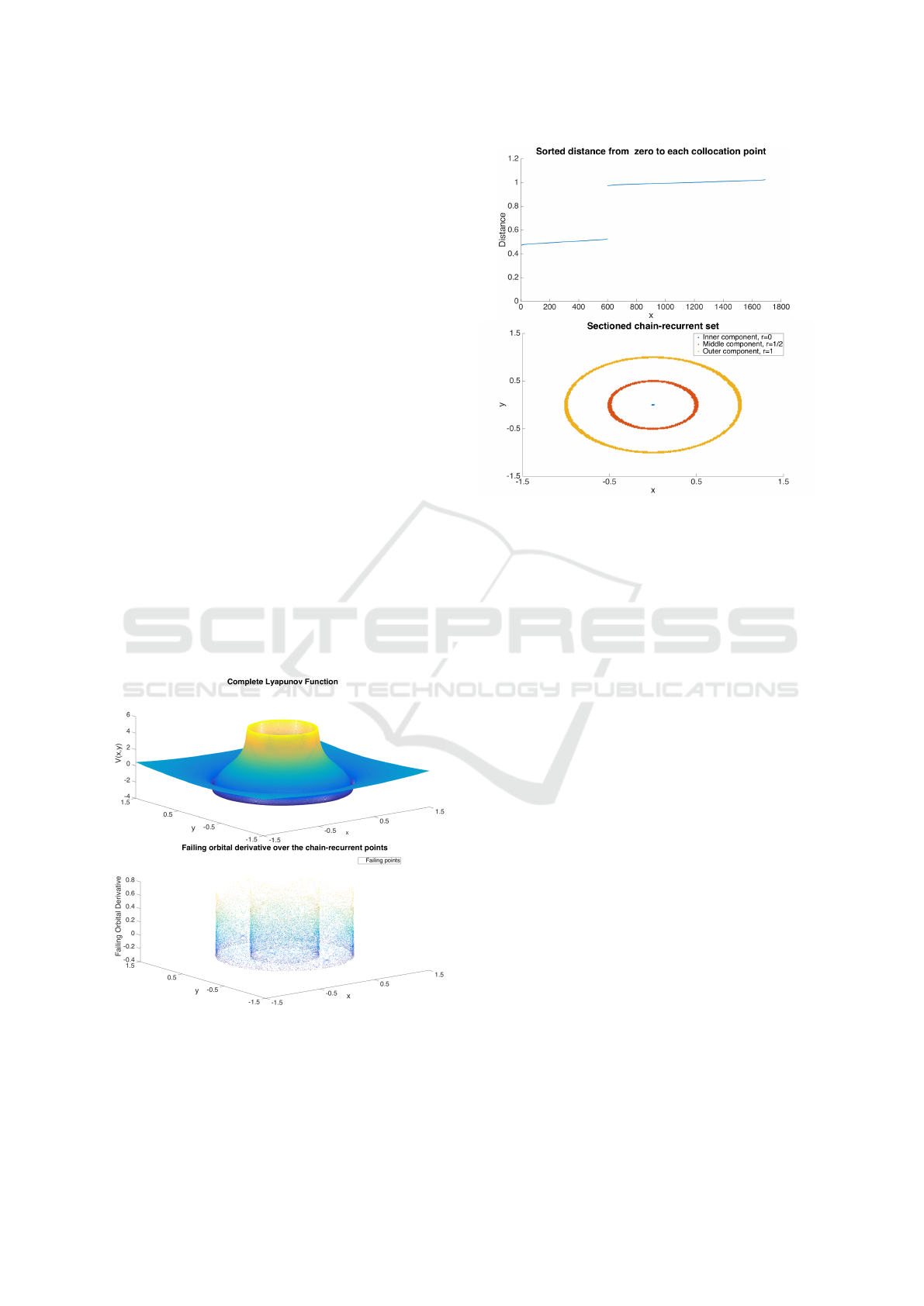
Figure 1: Upper figure: Complete Lyapunov function at the
initial iteration for system (7). Lower figure: Values of the
orbital derivative over the chain-recurrent set.
The distances that allowed to classify the orbits
are shown in Fig. 2, note that these examples are com-
puted with the original iteration ite=0.
Figure 2: Upper: Sorted distance of each failing collocation
point from zero for system (7). Lower: Three identified sets
within the chain-recurrent set for (7). These sets are formed
with two orbits with radii r = 1 and r = 1/2 and the failing
points around the origin.
In Fig. 2 there are two main gaps, giving three
connected components: The points near zero and the
two remaining orbits. This allows us to classify the
origin and the two orbits as subsets of the chain-
recurrent set for system (7), see Fig. 2.
3.2 Van der Pol Oscillator
System (8) is a two-dimensional form of the Van der
Pol oscillator. The system has an asymptotically sta-
ble periodic orbit and an unstable equilibrium at the
origin.

˙x
˙y

= f(x,y) =

y
(1 − x
2
)y − x

(8)
For computing the complete Lyapunov function
associated to system (8), we set α
Hexa-basis
= 0.05 over
the area defined by [−4.0, 4.0]
2
⊂ R
2
. The Wendland
function parameters used are (l,k,c) = (4, 2, 1), the
critical value γ = −0.5, and δ
2
= 10
−8
. The evalu-
ation grid was computed with the hexagonal subgrid
with parameter i
max
= 3.
The complete Lyapunov function at the initial
iteration and the orbital derivative over the chain-
recurrent set is shown in Fig. 3
Unlike system (7), the current system under anal-
ysis has only one periodic orbit which is not circular.
Fig. 4 allows to understand how Euclidean norm of
each element of the chain-recurrent set looks when
sorted in an increasing order.
ICINCO 2019 - 16th International Conference on Informatics in Control, Automation and Robotics
142

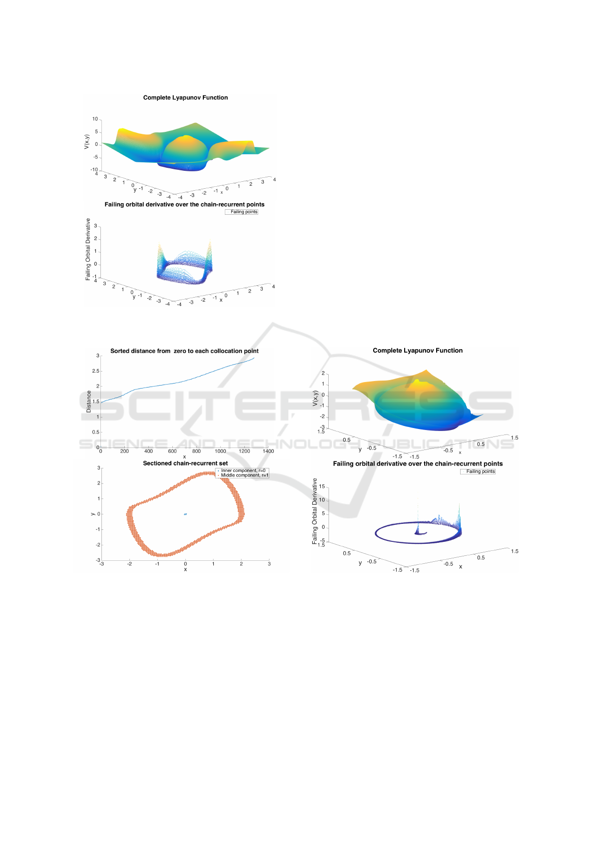
Figure 3: Upper figure: Complete Lyapunov function at the
initial iteration for system (8). Lower figure: Values of the
orbital derivative over the chain-recurrent set.
Figure 4: Upper: Sorted distance of each failing collocation
point from zero for system (8). Lower: Two identified sets
within the chain-recurrent set for (8).
3.3 Homoclinic Orbit
As in (Arg
´
aez et al., 2017a), we also consider here the
following example

˙x
˙y

= f(x,y) =

x(1 − x
2
− y
2
) − y((x − 1)
2
+ (x
2
+ y
2
− 1)
2
)
y(1 − x
2
− y
2
) + x((x − 1)
2
+ (x
2
+ y
2
− 1)
2
)

.
(9)
The origin is an unstable focus and the system has
an asymptotically stable homoclinic orbit at a circle
centred at the origin and with radius 1, connecting the
equilibrium (1,0) with itself.
We used the Wendland function ψ
4,2
for our com-
putations. Our collocation points were defined in the
region [−1.5, 1.5] × [−1.5,1.5] ⊂ R
2
with a hexag-
onal grid (4) with α
Hexa−basis
= 0.0125. In this ex-
ample, we have used the normalized method, i.e. we
replaced f by
ˆ
f as in (2) with δ
2
= 10
−8
, and we
used γ = −0.75. As before, the evaluation grid was
computed with the hexagonal subgrid with parameter
i
max
= 3.
The Lyapunov function at the initial iteration is
shown in Fig. 5 along with the orbital derivative over
the chain-recurrent set. The distances that allow to
classify the components are shown in Fig. 6 along
with the classified orbits. As with the Van der Pol
oscillator, we have two connected components: the
equilibrium at the origin and the unit circle. The equi-
librium at the origin is clearly over-estimated.
Figure 5: Upper figure: Complete Lyapunov function at the
initial iteration for system (9). Lower figure: Values of the
orbital derivative over the chain-recurrent set.
It can be seen in the examples given for systems
(7), (8) and (9) that the connected components of
the chain-recurrent set are subsets of lower dimen-
sion than the state space. This was the main tool used
in our heuristic algorithm in (Arg
´
aez et al., 2019b).
However, there are obviously examples where this as-
sumption does not hold; we will see that our new al-
gorithm can easily cope with such examples.
Clustering Algorithm for Generalized Recurrences using Complete Lyapunov Functions
143

Figure 6: Sorted distance of each failing collocation point
from zero for system (9). Lower: These sets form an orbit
with radius r = 1 and the failing points around the origin for
system (9).
3.4 Two-dimensional Chain-recurrent
Set
We consider the system with right-hand side
f(x,y) =

xΓ(x,y) − y
yΓ(x,y) + x

with
Γ(x,y) =



(1 − x
2
− y
2
)
3
if x
2
+ y
2
< 1
0 if 1 ≤ x
2
+ y
2
≤ 4
(4 − x
2
− y
2
)
3
if x
2
+ y
2
> 4
(10)
The origin is an unstable equilibrium, and there is
a family of periodic orbits of radius [1, 2]. Hence, the
chain-recurrent set has two connected components:
the origin and the annulus between the circles of ra-
dius 1 and 2.
We used the Wendland function ψ
4,2
for our com-
putations and set our collocation points in the region
[−1.5,1.5] × [−1.5,1.5] ⊂ R
2
with a hexagonal grid
(4) with α
Hexa−basis
= 0.0163. In this example, we
have used the normalized method, i.e. we replaced f
by
ˆ
f as in (2) with δ
2
= 10
−8
, and we used γ = −0.97.
The evaluation grid was computed with the di-
rectional grid with parameter m = 11. The Lya-
punov function at the initial iteration is shown in
Fig. ?? along with the orbital derivative over the
chain-recurrent set. The distances that allowed to
classify the orbits are shown in Fig. 8 along with
the classified connected components. Our previous
heuristic algorithm (Arg
´
aez et al., 2019b) would not
have been able to classify this two-dimensional com-
ponent of the chain-recurrent set.
Figure 7: Upper figure: Complete Lyapunov function at the
initial iteration for system (10). Lower figure: Values of the
orbital derivative over the chain-recurrent set.
3.5 Three-dimensional Systems
Giving the nature of this algorithm, one could con-
sider to extend its application to three dimensional
systems. In fact, the algorithm is based on distances
from the origin regardless of the system’s dimension.
Therefore, the algorithm explained in Sec. 2 is also
valid for three dimensional systems, under the obser-
vation that now the distances from zero are measured
for points with three coordinates instead of two.
Let us consider the system


˙x
˙y
˙z


= f(x,y,z) =


µx − y − xz,
x + µy
−z + x
2
z + y
2


(11)
which has been introduced in (Chen and J. Shen,
2014); we use µ = 0.1. The area used to build
the collocation points is: [−0.7,0.7] × [−0.7,0.7] ×
[−0.4,0.4] with α = 0.039, γ = −0.25. This problem
was iterated 55 times.
Figure 9 shows the set of failing evaluation points,
characterizing the chain-recurrent set. that failed to-
gether with the set of collocation points that were
identify for our algorithm. It can be seen in the ex-
treme superior part of the figure, a collection of points
that were identify in the chain-recurrent set. How-
ever, no collocation points are associated to them in
ICINCO 2019 - 16th International Conference on Informatics in Control, Automation and Robotics
144

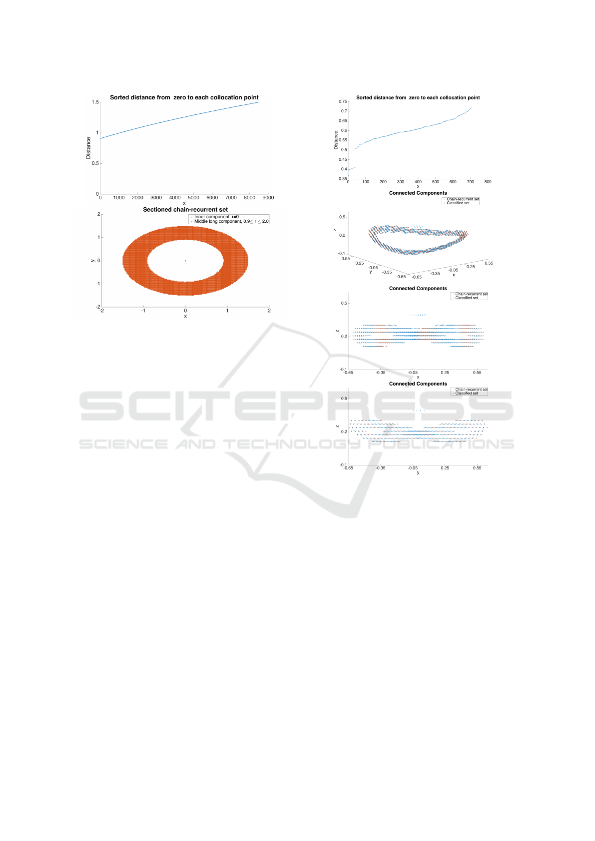
Figure 8: Upper: Sorted distance of each failing collocation
point from zero for system (10). Lower: Two identified
sets within the chain-recurrent set for (10). These sets are
formed with one large orbit with radius r ≤ 1.5 and r ≥ 0.9
and the failing points around the origin.
the classification because they belong to the bound-
ary of our domain. So, the subclassified collocation
points are only those that fail by the approximation.
A first step to clean the chain-recurrent set is to dis-
charge all points in the boundary of the domain.
4 CONCLUSIONS
In this contribution we have introduced an algorithm
capable of finding and classifying the different con-
nected components of the chain-recurrent set. The al-
gorithm works for arbitrary chain-recurrent sets and is
thus a major improvement from our previous heuristic
algorithm (Arg
´
aez et al., 2019b). Based on the algo-
rithm in this paper, we can now address the problem
of over-estimation of the chain-recurrent set in future
work, following the idea of (Arg
´
aez et al., 2019b).
ACKNOWLEDGEMENTS
The first author in this paper is supported by the Ice-
landic Research Fund (Rann
´
ıs) grant number 163074-
052, Complete Lyapunov functions: Efficient numer-
ical computation.
Figure 9: Upper first: Sorted distance of each failing col-
location point from zero for system (11). Upper second:
Identified set within the chain-recurrent set for system (11).
Lower first: Identified set within the chain-recurrent set for
system (11), xz plane. Lower second: Identified set within
the chain-recurrent set for system (11), yz plane. All figures
were obtained with 55 iterations.
REFERENCES
Arg
´
aez, C., Giesl, P., and Hafstein, S. (2017a). Analysing
dynamical systems towards computing complete Lya-
punov functions. In Proceedings of the 7th In-
ternational Conference on Simulation and Modeling
Methodologies, Technologies and Applications (SI-
MULTECH), pages 134–144. Madrid, Spain.
Arg
´
aez, C., Giesl, P., and Hafstein, S. (2018a). Computation
of complete Lyapunov functions for three-dimensional
systems. In Proceedings IEEE Conference on Deci-
sion and Control (CDC), 2018, pages 4059–4064. Mi-
ami Beach, FL, USA.
Arg
´
aez, C., Giesl, P., and Hafstein, S. (2018b). Compu-
Clustering Algorithm for Generalized Recurrences using Complete Lyapunov Functions
145

tational approach for complete Lyapunov functions.
In Dynamical Systems in Theoretical Perspective.
Springer Proceedings in Mathematics & Statistics. ed.
Awrejcewicz J. (eds)., volume 248.
Arg
´
aez, C., Giesl, P., and Hafstein, S. (2018c). Iterative
construction of complete Lyapunov functions. In Pro-
ceedings of the 8th International Conference on Sim-
ulation and Modeling Methodologies, Technologies
and Applications (SIMULTECH). Porto, Portugal.
Arg
´
aez, C., Giesl, P., and Hafstein, S. (2019a). Clustering
algorithm for generalized recurrences using complete
Lyapunov functions. ICCS 2019, Faro.
Arg
´
aez, C., Giesl, P., and Hafstein, S. (2019b). Improved
estimation of the chain-recurrent set. In IEEE Xplore
digital library. ACCEPTED. ECC 2019, Naples.
Arg
´
aez, C., Hafstein, S., and Giesl, P. (2017b). Wendland
functions a C++ code to compute them. In Proceed-
ings of the 7th International Conference on Simulation
and Modeling Methodologies, Technologies and Ap-
plications (SIMULTECH), pages 323–330. Madrid,
Spain.
Chen, H. and J. Shen, Z. Z. (2014). Existence and analytical
approximations of limit cycles in a three-dimensional
nonlinear autonomous feedback control system. J Syst
Sci Complex., 27:1158.
Conley, C. (1978). Isolated Invariant Sets and the Morse In-
dex. CBMS Regional Conference Series no. 38. Amer-
ican Mathematical Society.
Conley, C. (1988). The gradient structure of a flow I. Er-
godic Theory Dynam. Systems, 8:11–26.
Dellnitz, M. and Junge, O. (2002). Set oriented numeri-
cal methods for dynamical systems. In Handbook of
dynamical systems, Vol. 2, pages 221–264. North-
Holland, Amsterdam.
Hsu, C. S. (1987). Cell-to-cell mapping, volume 64 of Ap-
plied Mathematical Sciences. Springer-Verlag, New
York.
Hurley, M. (1995). Chain recurrence, semiflows, and gra-
dients. J Dyn Diff Equat, 7(3):437–456.
Hurley, M. (1998). Lyapunov functions and attractors in
arbitrary metric spaces. Proc. Amer. Math. Soc.,
126:245–256.
Iske, A. (1998). Perfect centre placement for radial basis
function methods. Technical Report TUM-M9809, TU
Munich, Germany.
Krauskopf, B., Osinga, H., Doedel, E. J., Henderson, M.,
Guckenheimer, J., Vladimirsky, A., Dellnitz, M., and
Junge, O. (2005). A survey of methods for computing
(un)stable manifolds of vector fields. Internat. J. Bifur.
Chaos Appl. Sci. Engrg., 15(3):763–791.
Lyapunov, A. M. (1907). Probl
`
eme g
´
en
´
eral de la stabilit
´
e
du mouvement. Ann. of math. Stud. 17. Princeton.
Ann. Fac. Sci. Toulouse 9, 203–474. Translation of
the russian version, published 1893 in Comm. Soc.
math. Kharkow. Newly printed: Ann. of math. Stud.
17, Princeton, 1949.
Lyapunov, A. M. (1992). The general problem of the sta-
bility of motion. Internat. J. Control, 55(3):521–790.
Translated by A. T. Fuller from
´
Edouard Davaux’s
French translation (1907) of the 1892 Russian orig-
inal.
P. Giesl C. Arg
´
aez, S. H. and Wendland, H. (2018).
Construction of a complete Lyapunov function using
quadratic programming. In Proceedings of the 15th
International Conference on Informatics in Control,
Automation and Robotics (ICINCO). SIMULTECH
2018, Porto.
Wendland, H. (1998). Error estimates for interpolation by
compactly supported Radial Basis Functions of mini-
mal degree. J. Approx. Theory, 93:258–272.
ICINCO 2019 - 16th International Conference on Informatics in Control, Automation and Robotics
146