
A Parallel Bit-map based Framework for Classification Algorithms
Amila De Silva and Shehan Perera
Department of Computer Science & Engineering, University of Moratuwa, Katubedda, Sri Lanka
Keywords:
Data Mining, Classification, Bitmaps, Bit-Slices, GPU.
Abstract:
Bitmaps are gaining popularity with Data Mining Applications that use GPUs, since Memory organisation and
the design of a GPU demands for regular & simple structures. However, absence of a common framework
has limited the benefits of Bitmaps & GPUs mostly to Frequent Itemset Mining (FIM) algorithms. We in
this paper, present a framework based on Bitmap techniques, that speeds up Classification Algorithms on
GPUs. The proposed framework which uses both CPU and GPU for Algorithm execution, delegates compute
intensive operations to GPU. We implement two Classification Algorithms Na
¨
ıve Bayes and Decision Trees,
using the framework, both which outperform CPU counterparts by several orders of magnitude.
1 INTRODUCTION
Long before the advent of Data Mining, Bitmaps have
been used in analytical queries. Bitmap based tech-
niques have been used when evaluating long predi-
cate statements and different varieties of Bitmap in-
dices have been proposed as early as 1997(O’Neil
and Quass, 1997). In certain studies like(Sinha and
Winslett, 2007), authors have proposed methods to
store data in Bitmaps which enable querying scientific
data,that mainly consists of floating-point numbers,
efficiently. Bitmaps have been used for different Ap-
plications from a long time, but mainly Bitmaps have
been used as a complementary index, not as a com-
plete data structure. An instance where Bitmaps have
been considered from the perspective of a data struc-
ture is(Fang et al., 2009), where Bitmaps have been
applied for a Frequent Itemset Mining(FIM)(Chee
et al., 2018) algorithm.
The organization and the processing done with
Bitmaps makes it a natural candidate for FIM algo-
rithms. In FIM algorithms such as Apriori(Agrawal
and Srikant, 1994), individual itemsets are mapped
into distinct Bitmaps so that generation of new item-
sets can be easily done by intersecting Bitmaps.
Showing that Bitmaps aren’t limited to FIM algo-
rithms, authors have implemented a Decision Tree
algorithm using Bitmaps in (Favre and Bentayeb,
2005), which uses Bitmap indices residing on a
database to obtain counts needed to build the tree.
Similar to Bitmaps, another emerging technique
being increasingly used in Data Mining is process-
ing with GPUs. GPUs are being increasingly consid-
ered for Data Mining algorithms due to their ability
to execute algorithms in parallel and also due to the
repetitive nature of Data Mining workloads. In stud-
ies (Fang et al., 2009; Silvestri and Orlando, 2012;
Chon et al., 2018),Bitmaps have been used on GPUs
to accelerate FIM algorithms,but the type of process-
ing they do can be extended to other algorithms.
In this study we are exploring the ability to use
Bitmap processing for Classification Algorithms. We
propose a Bitmap-based CPU-GPU hybrid frame-
work for Classification Algorithms, which uses two
Bitmap representations, Bitmaps and BitSlices. We
also propose a Batching technique which limits num-
ber of kernel invocations and improves performance
significantly. To prove our hypothesis, we imple-
ment two algorithms Na
¨
ıve Bayes and Decision Tree
using both the representations and show that signif-
icant speedups can be obtained with the proposed
techniques. In the experiments we perform with real
world datasets, we obtain average speed ups of 30 and
3 for Na
¨
ıve Bayes and Decision Trees respectively.
2 RELATED WORK
In this section, we briefly review related work on Data
Mining frameworks which uses GPUs, Distributed
Algorithms proposed for Classification Algorithms
and use of Bitmaps in Data Mining algorithms.
De Silva, A. and Perera, S.
A Parallel Bit-map based Framework for Classification Algorithms.
DOI: 10.5220/0007931202590266
In Proceedings of the 8th International Conference on Data Science, Technology and Applications (DATA 2019), pages 259-266
ISBN: 978-989-758-377-3
Copyright
c
2019 by SCITEPRESS – Science and Technology Publications, Lda. All rights reserved
259

2.1 GPU Frameworks for Data Mining
Applications
In work done by B
¨
ohm et al.(B
¨
ohm et al., 2009), a
framework, which uses an optimised index to speed
up similarity join operations, has been proposed . By
expressing two clustering algorithms DBSCAN and
K-Means with similarity join, they have obtained sig-
nificant speed ups over CPU counterparts. Their pro-
posed technique has so far been applied to Clustering
Algorithms,even they claim that the technique can be
applied for other Algorithms.
The framework proposed by Fang et al. ,
GPUMiner (Fang et al., 2008) is much closer to what
we are doing, in the sense that it uses Bitmaps for
all algorithms supported by the framework. They use
both Horizontal and Columnar Data layouts and fa-
cilitates multiple algorithms falling into different cat-
egories. In GPUMiner, Bitmaps are being used for
different types of operations. In Apriori, Bitmaps
are utilised to represent unique itemsets and are used
while computing support and generating candidates.
From the perspective of Apriori Algorithm, this is a
core operation, since it’s the most compute intensive
step. But in clustering algorithms, Bitmaps are used
for tracking the identity of different data points. This
operation can only be considered as a supporting task,
because it doesn’t directly involve with calculating
distance, which is the compute intensive operation in
Clustering Algorithms.
Another study that proposes a framework for Data
Mining algorithms is (Gainaru and Slusanschi, 2011),
where the framework provides core functionalities
like handling data transfers and scheduling while giv-
ing the flexibility to extend/perform algorithm spe-
cific changes. With their approach of unifying data
transfers, they have been able to use optimization
techniques applied for one algorithm to improve an-
other. But they haven’t been able to surpass speed ups
that can be obtained with Bitmaps.
In work done by Jian et al.(Jian et al., 2013), they
propose 3 main techniques which improves process-
ing on GPUs. These techniques address three recur-
ring operations in Data Mining applications. Their so-
lution to one such problem which is processing high-
dimensional data, is to follow column-wise process-
ing. This approach enables GPU to apply sequential
addressing reduction(Harris, 2016), which is the same
technique we are using in our study.
2.2 Parallel Data Mining Algorithms
In (Fang et al., 2009) authors present two efficient
GPU based Apriori algorithms that use Bitmaps, one
running solely using Bitmaps and another using a Trie
to do candidate generation. Support counting part in
both algorithms is delegated to the GPU and count-
ing support of a single itemset is handled by a sin-
gle thread block. For support counting both the vari-
ants rely on Bitmap representation. Another couple
of studies where GPUs are used in FIM algorithms
are (Silvestri and Orlando, 2012) and (Chon et al.,
2018). In (Silvestri and Orlando, 2012), algorithm de-
fers using GPU until all the frequent itemsets fit into
device memory, which prevents frequent data trans-
fers between host and the device. With this technique,
they’ve been able to observe significant speed ups. In
(Chon et al., 2018) authors have explored the possibil-
ity of using multiple GPUs while exploiting the abil-
ity to compute a partial sum in each thread block. In
both the studies, Bitmaps have been used for storing
Frequent Itemsets.
Recently, Viegas et al.(Andrade et al., 2013) im-
plemented Na
¨
ıve Bayes algorithm on GPUs. In their
implementation they’ve used a compact data structure
indexed by terms, which has helped them to minimize
memory consumption. The compact structure being
used, help them to perform model building in paral-
lel, allowing them to achieve 35 times speed up over
sequential CPU execution.
One of the earliest methods for building a De-
cision tree in parallel has been proposed in (Shafer
et al., 1996), where records are distributed among
multiple processors. Algorithm SPRINT is an im-
provement over SLIQ(Mehta et al., 1996), and has
adopted many characteristics from SLIQ. SPRINT
proposes a parallel tree building technique which dis-
tributes computation by delegating each node to a dif-
ferent processor.
But these algorithms are designed on multipro-
cessor systems, where each processor has access to
a dedicate memory and a hard disks. At a concep-
tual level, data organisation and processing followed
in our framework for Decision Tree, is similar to the
methods used in SPRINT(Shafer et al., 1996).
Techniques proposed in(Shafer et al., 1996) have
been adopted in CudaTree(Liao et al., 2013) which
is a GPU based implementation. In addition to the
characteristics borrowed from SPRINT, another ap-
proach CudaTree(Liao et al., 2013) explores is, blend-
ing task parallelism and data parallelism by switching
between two different modes of tree building.
There are couple of algorithms proposed for build-
ing Random forests on GPUs. Algorithm proposed in
(Amado et al., 2001) exploits task parallelism by task-
ing each core with building a single tree. Authors are
claiming that the algorithm works best when lot of
parallel trees are built.
DATA 2019 - 8th International Conference on Data Science, Technology and Applications
260
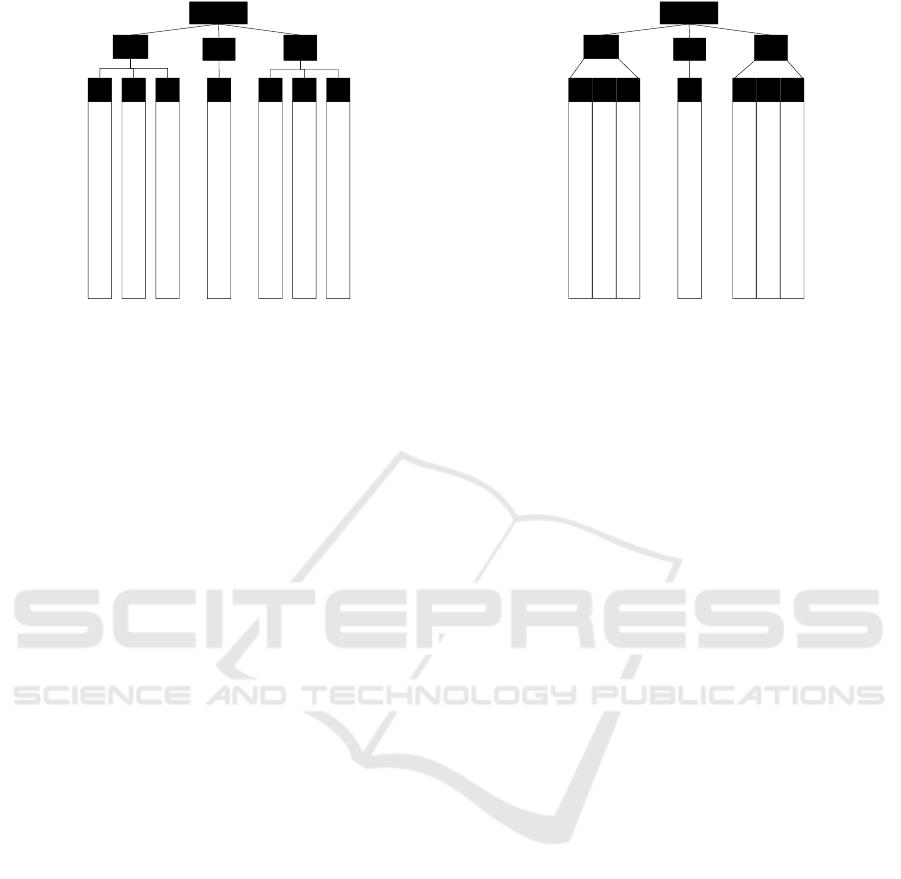
1
1
0
1
0
1
1
1
..
1
1
A1
B
1
B
2
1
0
1
1
1
1
0
0
..
1
1
1
1
1
0
1
1
0
1
..
0
1
B
3
Ai
B
k
...
1
1
0
1
0
1
1
1
..
1
1
An
B
1
B
k
...
1
0
1
1
1
0
1
0
..
1
0
B
m
Dataset
Figure 1: Dataset represented using Bitmaps.
3 DESIGN AND
IMPLEMENTATION
This section mainly describes the design and imple-
mentation of our framework. We talk in-depth about
the two Bitmap variants supported by the framework,
Bitmaps and BitSlices, highlighting each area they
can be optimally used in. We also talk about the two
algorithms implemented using the framework, Na
¨
ıve
Bayes and Decision tree, detailing about types of pro-
cessing needed for each algorithm and showing how
our framework provides those. Then we move onto
discuss how batching is implemented and how it re-
duces running time of algorithms.
3.1 BitSlice And Bitmap
Representations
The BitSlice and Bitmap representations we are talk-
ing about are widely known index schemes available
in literature. However in the scope of our work, rather
than using as index schemes we are using those to
store actual underlying data. Before converting to ei-
ther format, data is first arranged into a column-major
format.
The Bitmap representation is similar to Value-List
indices proposed in (O’Neil and Quass, 1997). If
Dataset D can be represented as a collection of At-
tributes {A
1
, A
2
, A
3
, . . . , A
n
} where each Attribute has
| R | number of elements and cardinality of attributes
(the number of distinct values) in each attribute can be
expressed as {C
1
, C
2
, C
3
, . . . , C
n
}, then we can define
Bitmap and BitSlice representations as below.
The Bitmap representation is a Set B
{B
1
, B
2
, B
3
, . . . , B
n
} where B
i
is the set of Bitmaps
corresponding to Attribute A
i
. B
i
can be expressed by
a set of Bitmaps {b
i,1
, b
i,2
, b
i,3
, . . . , b
i,m
} where b
i,j
is
1
0
0
1
1
1
1
1
..
1
1
A1
2
2
2
1
0
0
1
1
1
1
0
0
..
1
1
1
1
1
0
1
1
0
1
..
0
1
2
0
Ai
2
k
...
An
1
0
0
1
0
1
0
1
..
1
1
2
m
2
k
...
0
1
1
1
1
0
1
0
..
1
0
2
0
Dataset
Figure 2: Dataset represented using BitSlices.
a vector of bits consisting of either ones or zeros and
m = C
i
. Size of each Bitmap is equal to the number
of records in the Dataset or | b
i,j
|=| R |. Assuming
that distinct values in A
i
can be expressed by the set
{a
i,1
, a
i,2
, a
i,3
, . . . , a
i,m
}, then k
th
bit in b
i,j
is set to one
only if k
th
value in A
1
is equal to a
i,j
. This way k
th
value will be set to 1 only in one bitmap. Loosely
defining, b
i,j
gives the locations a
i,j
is appearing in
dataset. Fig. 1 gives a graphical illustration of the
Bitmap representation. As depicted in the Figure,
attribute A
1
has 3 distinct values, hence the 3 Bitmaps
B
1
,B
2
and B
3
. Similarly, A
n
has m attributes which
are shown by the Bitmaps B
1
, . . . , B
m
.
BitSlice representation of Dataset D can be de-
fined by making slight modification to the previous.
Assuming attribute A
i
can be represented as a binary
number with N+l bits, the Bit sliced representation of
A
i
is an ordered list of bitmaps b
i,N
, b
i,N-1
, . . . , b
i,1
,
b
i,0
where these Bitmaps are called the BitSlices. If
A
i
[k] denotes, k
th
element in Attribute A
i
and the bit
for row k in bit-slice b
i,j
by b
i,j
[k] then the values for
b
i,j
[k] are chosen so that
A
i
[k] =
N
∑
i=1
b
i,j
[k] × 2
i
(1)
Note that we determine N in advance so that
the highest-order bit-slice b
i,N
is non-empty. Usu-
ally N is selected so that N = log
2
(max(A
i
)). Bit-
Slice representation of the Dataset D is the set B
{B
1
,B
2
,B
3
,. . . ,B
n
} where B
i
is the BitSlice represen-
tation of Attribute A
i
. Fig. 2 illustrates the Dataset
represented in BitSlices. Note that all the values in
column A
1
are represented by three BitSlices, which
means that the maximum value in A
1
is 7. Simi-
larly, A
n
is represented by m BitSlices, meaning that
2
m+1
− 1 is the maximum values present in the col-
umn.
Even we define a single Bitmap as a vector of
bits, when implementing it programatically, bits are
A Parallel Bit-map based Framework for Classification Algorithms
261
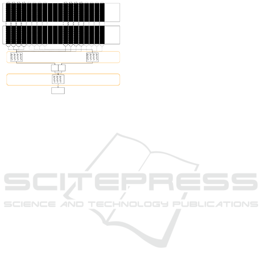
n1 n2
n1+n2
Intersect &
count
summation
101100101...1
101100101...1
101100101...1
101100101...1
101100101...1
101100101...1
101100101...1
101100101...1
101100101...1
101100101...1
...
101100101...1
101100101...1
101100101...1
101100101...1
101100101...1
101100101...1
101100101...1
101100101...1
Bitmap 2
101100101...1
101100101...1
101100101...1
101100101...1
101100101...1
101100101...1
101100101...1
101100101...1
101100101...1
101100101...1
...
101100101...1
101100101...1
101100101...1
101100101...1
101100101...1
101100101...1
101100101...1
101100101...1
Bitmap 1
& & & & & & & & & & & &
Cycle 2
& & & &
Block 1
Block 2
Cycle 1
Figure 3: Bitmap intersection & counting on GPU.
grouped into chunks of 64 and is usually stored as an
array of unsigned long (ulong) literals. Then Bitmap
intersection would reduce into performing bitwise
AND between two ulong arrays.
3.2 Bitmap and BitSlice Processing
When data is represented with BitSlices/Bitmaps, ap-
plying filters and searching for data elements needs
Bitmap manipulation. Since data is encoded, obtain-
ing a count with a Bitmap structure isn’t straight-
forward. Framework provides a range of core al-
gorithms, which manipulates the underlying Bitmap
structure and give a result for a query. Co-
occurenceCount is such a core algorithm which would
count the co-occurrence of two numbers among two
columns. Since Co-Occurrence counting makes up
the most basic processing in the framework, we’ll first
show how this operation is performed with Bitmaps
& BitSlices. Co-occurence counting is frequently
used when populating contingency tables. While im-
plementing Both Na
¨
ıve Bayes and Decision Tree we
used a contingency table to perform computations.
Co-OccurenceCount is implemented as a kernel
and at the start of the kernel,the entire Dataset gets
transferred to the Device memory. Since GPU is only
transferring result of a computation, there won’t be
any major data transfers from GPU to CPU.
The basic unit in either of these representations is
a Bitmap, which is kept as ulong vector. Result of
an intersection produces another Bitmap, count of 1
of which can be obtained using popcount instruction
available in CUDA. Since both Bitmaps and BitSlices
are representationally similar, we’ll explain in detail
about Bitmap processing and then briefly talk about
BitSlices.
3.2.1 Processing with Bitmaps
With the Bitmap representation each attribute is a
collection of Bitmaps, so counting co-occurrence be-
tween two attributes would involve intersecting and
counting Bitmaps.
In sequential addressing reduction(Harris, 2016)
, each GPU core would work on the same intersec-
tion and count operation, regardless of the GPU mul-
tiprocessor they belong to. Each thread is in charge
of an interleaved portion of the Bitmap, in such a way
that threads having consecutive indexes work on con-
secutive parts of the Bitmap. In Fig. 3 we provide
a visualisation of the Bitmap intersection. Bitmap 1
and Bitmap 2 are two ulong arrays residing in GPU’s
main memory. In Cycle1 each block will be pro-
cessing the set of elements located to the left of the
Bitmaps.Block 1 will be processing elements demar-
cated by broken lines while Block 2 will be process-
ing elements with dotted lines. Each thread in the
block will pick an index and read two elements lo-
cated at that position from two Bitmaps. Intersec-
tion and counting would happen in each thread and
would get aggregated by the block level when writ-
ing to shared memory. At the end of Cycle 1, Block 1
will write the aggregation of 4 elements located to
the very left of the Bitmap and Block 2 will simi-
larly write down aggregation of the next 4.In Cycle 2,
both the blocks will pick a different portion of the
same Bitmaps. Block 2 will be picking the last 4 ele-
ments to the right, the ones marked with dotted lines
and Block1 will pick next 4 elements from the end
marked with broken lines. The value n1 provided by
Block 1 at the end of Cycle 2 is the aggregation of all
elements processed by Block 1. Similarly n2 is the
aggregation of all elements processed by Block 2. If
there are n blocks, then an array of n will be written
to Global memory, each with the aggregation of all
elements processed by each block. Summing up this
array would give the result for the entire Bitmap.This
is usually done by running a summing kernel provid-
ing the array with partial sums as the input.
The Algorithm BitmapCo-OccuranceCountGPU
shows the code for this Bitmap intersecting kernel.
Here col1 and col2 are the respective columns (at-
tributes) represented in Bitmaps needed for the inter-
section. Each column can be thought of as an array of
Bitmaps. Since we are only representing categorical
data with Bitmaps, a single category value would have
a unique Bitmap.index1 and index2 are the indices of
the first and second category values respectively. We
also pass the length which gives the number of ulong
literals in a Bitmap.
BitmapCo-OccuranceCountGPU (col1,col2,length,
DATA 2019 - 8th International Conference on Data Science, Technology and Applications
262

index1,index2,output)
tid <- threadIdx.x
i <- blockIdx.x x blockSize + threadIdx.x
gridSize <- blockSize x gridDim.x
sdata <- initialize shared memory
mySum <- 0
bitwise <- !0
while i < length:
bitwise <- col1[index1][i] &
col2[index2][i]
mySum <- mySum + _popcll(bitwise)
i <- i + gridSize
endwhile
sdata[tid] <- mySum
....
if tid == 0:
output[blockIdx.x] <- mySum
endif
We first initialise internal state variables by get-
ting Block and Thread configurations. The variables
threadIdx and blockIdx are set by CUDA environment
based on parameters we set while invoking the ker-
nel. Since this kernel is invoked by each thread, each
thread needs to select a non-overlapping portion of the
Bitmap. That’s why the variable i is determined using
blockIdx and threadIdx. Once we initialize variables
properly, we do a Bitmap intersection in line 9. A sin-
gle thread may work on multiple portions in different
iterations. To facilitate this, we keep increasing i by
the size of the Grid (i.e the number of blocks). We’ve
also omitted the part which performs block-wise ag-
gregation. The kernel would only write to the global
memory at the time of finishing kernel invocation, and
at other times it would only do reads. When doing
reads, consecutive threads will be read from adjacent
memory locations so the accesses are coalesced. And
when writing to shared memory, a sequential address-
ing method is followed to avoid bank conflicts.
3.2.2 Processing with BitSlices
Processing with BitSlices is very much similar to pro-
cessing Bitmaps, main difference being having to load
all the BitSlices belonging to the two attributes as op-
posed to reading the two particular Bitmaps.
BitSliceCo-OccuranceCountGPU (col1,col2,length,
val1,val2,col1_bitmaps,col2_bitmaps,output)
Initialising ...
while i < length:
bitwise <- !0
for k <- 0 to col1_bitmaps - 1:
if val1 & (1 << k):
bitwise <- bitwise & col1[k][i]
else:
bitwise <- bitwise & !col1[k][i]
endif
endfor
for k <- 0 to col2_bitmaps - 1:
if val2 & (1 << k):
bitwise <- bitwise & col2[k][i]
else:
bitwise <- bitwise & !col2[k][i]
endif
endfor
i <- i + gridSize
mySum <- mySum + _popcll(bitwise)
endwhile
sdata[tid] <- mySum
....
if tid == 0:
output[blockIdx.x] <- mySum
endif
Intersection with BitSlices are done in a fashion
similar to the algorithms described in Algorithm 4.2
(O’Neil and Quass, 1997). Algorithm BitSliceCo-
OccuranceCountGPU show the BitSlice intersecting
kernel running on GPU. In addition to the parameters
passed in BitmapCo-OccuranceCountGPU, we pass
the number of Bitmaps in each column (indicated by
col1 bitmaps&col2 bitmaps)and a pointer to output
array residing in the Global Memory. BitSlice Inter-
section looks a bit complex compared to Bitmap Ker-
nel, since there’s loop running to select the number.
In Bitmap Kernel we didn’t have to explicitly pass the
category values, but for BitSlices we need to do so,
since it’s based on those values intersection is done.
Similar to Bitmaps, once the intersecting and
counting is done, a block level reduction happens,
which is followed by a global reduction. The only
noticeable difference between the two representations
is that, in Bitmap representation a Bitmap is read-
ily available for an attribute value, but in BitSlices it
needs to be generated in the kernel as computation
happens.
3.2.3 Batching Operations
Usually arithmetic intensity of a Bitmap intersection
is low. To produce intersection of two Bitmaps, two
global reads have to be made. This makes the kernel,
a bandwidth sensitive one since a larger proportion
of time is spent in transferring Bitmaps from global
memory. With batching we'll be reading four Bitmaps
to produce four resulting Bitmaps. In the traditional
reduction phase, which follows counting operation,
count is kept in an integer. But in the batched mode
we are using int4, which easily allows us to keep four
pattern counts. However before transferring results to
host's side they need to be mapped with proper inte-
gers.
A Parallel Bit-map based Framework for Classification Algorithms
263
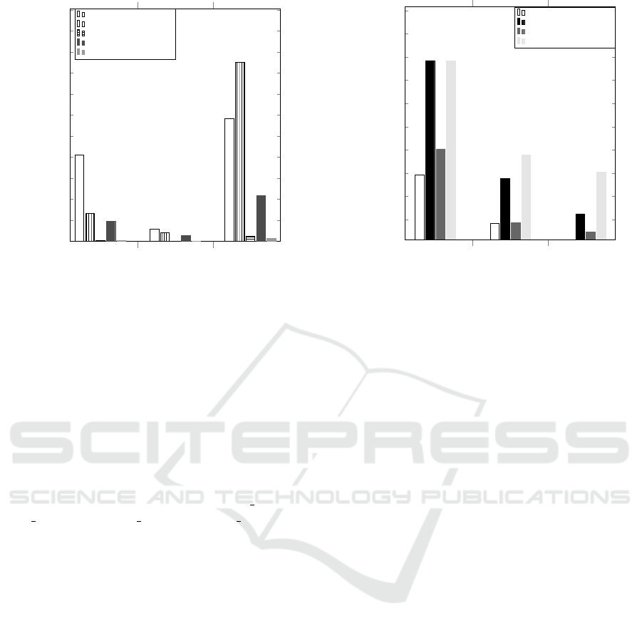
USCensus
PokerHand
KDDCUP
0.5
1
1.5
2
2.5
3
3.5
4
4.5
5
5.5
·10
6
2.06 · 10
6
2.87 · 10
5
2.92 · 10
6
6.71 · 10
5
2.15 · 10
5
4.26 · 10
6
23,348.4
7,624.2
1.3 · 10
5
4.82 · 10
5
1.39 · 10
5
1.08 · 10
6
23,386.8
6,000.8
72,358.4
Running Time(µs)
Standard-CPU
BitSlices-CPU
BitSlices-GPU Batched
Bitmaps-CPU
Bitmaps-GPU Batched
1
Figure 4: Execution times with Different Datasets Results
for Na
¨
ıve Bayes.
3.2.4 Implementing Algorithms on the
Framework
Both Na
¨
ıve Bayes and Decision Trees have been
implemented by using counts returned from Co-
OccurrenceCount kernels. For both the Algorithms
we used the implementation provided by weka (Wit-
ten et al., 2011). When an algorithm starts, it ini-
tializes a two-dimensional matrix at Device’s space,
transfers Dataset to the device and starts invoking
kernels. It’s to this matrix, the counts will be writ-
ten. The 2D Matrix has cells equal to att values ×
class values, where att values and class values rep-
resent cardinality of the test attribute and the class
attribute respectively. When using non-batched ker-
nels, each kernel invocation counts a single pattern
requiring that many invocations equal to the number
of cells. The batched mode can count four patterns at
once, so depending on the Dataset, a minimum of one
fourth of the invocations will happen.
4 PERFORMANCE EVALUATION
To evaluate performance of the framework, and to as-
sess correctness of algorithms, we present experimen-
tal results. Since our primary target is to measure per-
formance gains obtained by Bitmap and BitSlice vari-
ants on GPUs, results are compared with CPU vari-
ants which use those representations.
For experiments we used three Datasets available
in UCI machine learning repository (Dua and Graff,
2017), USCensus(b23, 1990), which is a categorical
dataset with 68 attributes and two million rows, Pok-
erHand(b24, 1990), which also is another categori-
USCensus
PokerHand
KDDCUP
20
30
40
50
60
70
80
90
100
110
39.41
18.54
11.51
88.43
37.7
22.52
50.44
18.75
14.77
88.29
47.9
40.39
Speed up
BitSlices-GPU
BitSlices-GPU Batched
Bitmaps-GPU
Bitmaps-GPU Batched
3
Figure 5: Speedup over Standard-CPU on different
Datasets.
cal dataset with 11 attributes and one million rows
and KDDCup99 dataset(b25, 1999). Most attributes
in KDDCup were real, due to which we had to split
those into ranges and create discrete categories.
In the following subsections we present experi-
ments performed and the criteria used in evaluating
algorithms.
4.1 Experimental Setup
All experiments were performed on a computer with
Intel Core 17-2600 CPU at 3,40GHz, with Hyper-
Threading, 16GB of main memory, and equipped
with a GeForce GTX480 graphics card. The GPU
consists of 15 SIMD multi-processors, each of which
has 32 cores running at 1.4 GHZ. The GPU memory
is 1.5 GB with the peak bandwidth of 177 GB/sec.
The goal of following tests is to assess perfor-
mance of two Na
¨
ıve Bayes implementations for GPU,
with respect to CPU implementations. We mainly
performed the test by using different datasets and
recording execution time of each variant. Accuracy
of the models were verified by comparing estimator
values set during each execution. For the experiments
we used 7 different implementations which are sum-
marized below.
• Standard-CPU - Unmodified implementation pro-
vided by Weka.
• BitSlice-CPU - Algorithm that uses Bitslices,
which runs on the CPU.
• Bitmap-CPU - An implementation running on
CPU using a Bitmap representation.
• Bitmap-CPU - An implementation running on
CPU using a Bitmap representation.
DATA 2019 - 8th International Conference on Data Science, Technology and Applications
264
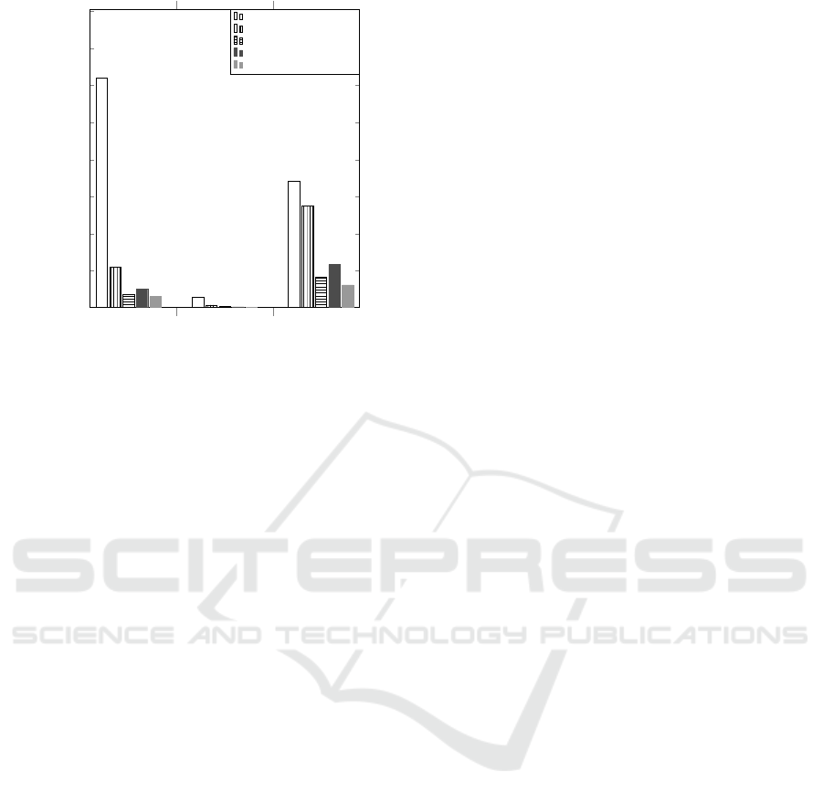
USCensus
PokerHand
KDDCUP
0.5
1
1.5
2
2.5
3
3.5
4
·10
7
3.1 · 10
7
1.45 · 10
6
1.71 · 10
7
5.52 · 10
6
3.95 · 10
5
1.37 · 10
7
1.78 · 10
6
2.4 · 10
5
4.18 · 10
6
2.55 · 10
6
1.64 · 10
5
5.85 · 10
6
1.56 · 10
6
1.12 · 10
5
3.12 · 10
6
Running Time(µs)
Standard-CPU
BitSlices-CPU
BitSlices-GPU Batched
Bitmaps-CPU
Bitmaps-GPU Batched
4
Figure 6: Execution times for Decision Tree with Different
Datasets.
• Bit-Slices GPU - The variant using Bit-Slices,
which runs on GPU.
• Bit-Slices GPU Batched - The same variant as
above, which performs operations in batches.
• Bitmap GPU - An implementation running on
GPU which uses Bitmaps.
• Bitmap GPU Batched - The bitmap variant run-
ning on GPU
running operations in batches.
In Fig. 4 we show the comparison with different
datasets, according to which we can see a clear differ-
ence between CPU and GPU variants. While measur-
ing time we only measured the time taken to build the
model. Transfer times were excluded because a trans-
fer would be done only once for multiple executions
and can be considered as a one time operation. The
graphs show an average time which is the average of
six iterations.
Fig. 5 shows the Speed ups for GPU variants, ob-
tained against Standard-CPU. This highlights the dif-
ference between batched and non-batched modes. In
all cases, batched variants report as twice as much
speed up when compared to the non-batched coun-
terpart. Further, an interesting observation can be
made with USCensus dataset. When comparing non-
batched executions for BitSlices and Bitmaps, in all
three Datasets Bitmap variant has given a better speed
up than the BitSlice variant. But such a difference
cannot be observed between batched variants for US-
Census. Both BitSlice-Batched and Bitmap-Batched
are showing similar speedups in USCensus. While
looking into the Dataset we found that, there are many
attributes having less than 4 distinct values. In the
non-batched mode, Bitmap based algorithm would
read two bitmaps to produce result of a single inter-
section, but to produce the result for the same inter-
section, BitSlice algorithm would read 4 BitSlices.
In batched mode, both the variants will be reading
4 Bitmaps to produce 4 results. Since memory ac-
cesses are more uniform in batched mode, BitSlice
and Bitmap algorithms run equally fast.
4.2 Results for Decision Trees
For Decision Tree algorithm, we ran a subset of the
above tests using the same three datasets. Same steps
followed for Na
¨
ıve Bayes were used while running
the experiments and verifying model accuracy. Re-
sults obtained for Decision Trees are shown in 6.
However, we didn’t execute non-batched modes for
Decision Trees, since batched mode itself wasn’t giv-
ing a considerable speed up. While implementing De-
cision Trees, we had to handle additional complexity
of maintaining partitions. It’s the approach we took in
handling partitions gave us considerable small perfor-
mance gains. Still the GPU variants finish faster than
CPU ones, but the speedups are very modest.
5 CONCLUSIONS
In this paper we focused on using Bitmap techniques
for classification algorithms. We showed that FIM al-
gorithms use Bitmaps on GPUs to perform compu-
tations in parallel. Then we showed that by separat-
ing out model building phase from the phase which
iterates through the Dataset , we can use Bitmap
based structures to speed up Algorithm execution.
The framework we proposed, represents Data with
Bitmaps and provides kernels to manipulate Bitmap
based structure. We also propose a batching technique
which enables performing multiple counting opera-
tions in a single kernel. By implementing two al-
gorithms, Na
¨
ıve Bayes and Decision Trees, we show
that proposed model can be used to implement, Clas-
sification algorithms. With the Datasets used in our
experiments, we’ve been able to achieve a maximum
speed ups of 80 for Na
¨
ıve Bayes, and 19 for Decision
Trees, against the CPU implementation. With this we
show that Bitmaps can be used on GPUs to speed up
Classification Algorithms. Results for Decision tree
even though remains promising, aren’t as significant
as Na
¨
ıve Bayes. We feel that, Decision Trees can
be improved further, since the approach we followed
incurs frequent memory transfers between CPU and
GPU. Bitmap representation provided the best speed
up in all cases, giving an indication that it can be used
to speed up processing categorical datasets. BitSlices
A Parallel Bit-map based Framework for Classification Algorithms
265

can be considered as a generic representation, since it
can hold both categorical and numerical data and also
since it doesn’t significantly reduce speed when com-
paring with Bitmap representation. We believe the
work discussed in this paper would provide a ground
work for building a Bitmap based framework for Data
Mining algorithms in general.
REFERENCES
(1990). Poker hand data set. URL: https://archive.ics.uci.
edu/ml/datasets/Poker+Hand. Online; Accessed 16
March 2019.
(1990). Us census data (1990) data set. URL: https://archive.
ics.uci.edu/ml/datasets/US+Census+Data+(1990).
Online; Accessed 16 March 2019.
(1999). Kdd cup (1999). kdd cup 99 intrusion detec-
tion datasets. URL: http://kdd.ics.uci.edu/databases/
kddcup99/kddcup99.html. Online; Accessed 16
March 2019.
Agrawal, R. and Srikant, R. (1994). Fast algorithms for
mining association rules. In Proc. of 20th Intl. Conf.
on VLDB, pages 487–499.
Amado, N., Gama, J., and Silva, F. M. A. (2001). Par-
allel implementation of decision tree learning algo-
rithms. In Proceedings of the10th Portuguese Con-
ference on Artificial Intelligence on Progress in Arti-
ficial Intelligence, Knowledge Extraction, Multi-agent
Systems, Logic Programming and Constraint Solving,
EPIA ’01, pages 6–13, London, UK, UK. Springer-
Verlag.
Andrade, G., Viegas, F., Ramos, G. S., Almeida, J., Rocha,
L., Gonc¸alves, M., and Ferreira, R. (2013). Gpu-nb:
A fast cuda-based implementation of na
¨
ıve bayes. In
2013 25th International Symposium on Computer Ar-
chitecture and High Performance Computing, pages
168–175.
B
¨
ohm, C., Noll, R., Plant, C., Wackersreuther, B., and
Zherdin, A. (2009). Data Mining Using Graphics Pro-
cessing Units, pages 63–90. Springer Berlin Heidel-
berg, Berlin, Heidelberg.
Chee, C.-H., Jaafar, J., Aziz, I. A., Hasan, M. H., and Yeoh,
W. (2018). Algorithms for frequent itemset mining: a
literature review. Artificial Intelligence Review.
Chon, K.-W., Hwang, S.-H., and Kim, M.-S. (2018).
Gminer: A fast gpu-based frequent itemset mining
method for large-scale data. Information Sciences,
439-440:19 – 38.
Dua, D. and Graff, C. (2017). UCI machine learning repos-
itory.
Fang, W., Lau, K. K., Lu, M., Xiao, X., Lam, C. K., Yang,
P. Y., He, B., Luo, Q., S, P. V., and Yang, K. (2008).
Parallel data mining on graphics processors. Technical
report.
Fang, W., Lu, M., Xiao, X., He, B., and Luo, Q. (2009).
Frequent itemset mining on graphics processors. In
Proceedings of the Fifth International Workshop on
Data Management on New Hardware, DaMoN ’09,
pages 34–42, New York, NY, USA. ACM.
Favre, C. and Bentayeb, F. (2005). Bitmap index-based de-
cision trees. In Proceedings of the 15th International
Conference on Foundations of Intelligent Systems, IS-
MIS’05, pages 65–73, Berlin, Heidelberg. Springer-
Verlag.
Gainaru, A. and Slusanschi, E. (2011). Framework for map-
ping data mining applications on gpus. In 2011 10th
International Symposium on Parallel and Distributed
Computing, pages 71–78.
Harris, M. (2016). Optimizing parallel reduction in
cuda. URL: https://developer.download.nvidia.com/
assets/cuda/files/reduction.pdf. Online; Accessed 16-
Feb-2019.
Jian, L., Wang, C., Liu, Y., Liang, S., Yi, W., and Shi, Y.
(2013). Parallel data mining techniques on graphics
processing unit with compute unified device architec-
ture (cuda). J. Supercomput., 64(3):942–967.
Liao, Y., Rubinsteyn, A., Power, R., and Li, J. (2013).
Learning random forests on the gpu.
Mehta, M., Agrawal, R., and Rissanen, J. (1996). Sliq: A
fast scalable classifier for data mining. In Apers, P.,
Bouzeghoub, M., and Gardarin, G., editors, Advances
in Database Technology — EDBT ’96, pages 18–32,
Berlin, Heidelberg. Springer Berlin Heidelberg.
O’Neil, P. and Quass, D. (1997). Improved query per-
formance with variant indexes. In Proceedings of
the 1997 ACM SIGMOD International Conference on
Management of Data, SIGMOD ’97, pages 38–49,
New York, NY, USA. ACM.
Shafer, J. C., Agrawal, R., and Mehta, M. (1996). Sprint:
A scalable parallel classifier for data mining. In Pro-
ceedings of the 22th International Conference on Very
Large Data Bases, VLDB ’96, pages 544–555, San
Francisco, CA, USA. Morgan Kaufmann Publishers
Inc.
Silvestri, C. and Orlando, S. (2012). gpudci: Exploiting
gpus in frequent itemset mining. In 2012 20th Euromi-
cro International Conference on Parallel, Distributed
and Network-based Processing, pages 416–425.
Sinha, R. R. and Winslett, M. (2007). Multi-resolution
bitmap indexes for scientific data. ACM Trans.
Database Syst., 32(3).
Witten, I. H., Frank, E., and Hall, M. A. (2011). Data
Mining: Practical Machine Learning Tools and Tech-
niques. Morgan Kaufmann Publishers Inc., San Fran-
cisco, CA, USA, 3rd edition.
DATA 2019 - 8th International Conference on Data Science, Technology and Applications
266
