“ReLIC: Reduced Logic Inference for Composition” for Quantiﬁer

Elimination based Compositional Reasoning

Hao Ren

1 a

, Ratnesh Kumar

2 b

and Matthew A. Clark

3 c

Honeywell Aerospace Advanced Technology, 12001 Hwy 55, Plymouth, MN, U.S.A.

Department of Electrical and Computer Engineering, Iowa State University, Ames, IA, U.S.A.

Galois Inc., 444 E 2nd St, Dayton, OH, U.S.A.

Keywords:

Quantiﬁer Elimination, Compositional Veriﬁcation, System Property Composition.

Abstract:

We present our work on the role and integration of quantiﬁer elimination (QE) for compositional veriﬁcation.

In our approach, we derive in a single step, the strongest system property from the given component properties.

This formalism is ﬁrst developed for time-independent properties, and later extended to the case of time-

dependent property composition. The extension requires additional work of replicating the given properties

by shifting those along time so the entire time-horizon of interest is captured. We show that the time-horizon

of a system property is bounded by the sum of the time-horizons of the component properties. The system

initial condition can also be composed, which, alongside the strongest system property, are used to verify a

postulated system property through induction. The above approaches are implemented in our prototype tool

called ReLIC (Reduced Logic Inference for Composition) and demonstrated through several examples.

1 INTRODUCTION

Compositional reasoning is employed for scaling the

model-based veriﬁcation approaches for distributed

systems. The component-based compositional design

paradigm emphasizes the separation of concerns with

respect to the system design through a modular and

reuse based paradigm for deﬁning, implementing, and

composing components into systems.

For example, Unmanned Systems Autonomy Ser-

vices (UxAS) software system (Rasmussen et al.,

2016) consists of a collection of modular services that

interact via a common message passing architecture.

It provides a framework to construct and deploy soft-

ware services that are used to enable autonomous ca-

pabilities by ﬂexibly implementing autonomy algo-

rithms on-board Unmanned Aerial Vehicles (UAV)s

(Kingston et al., 2016). Veriﬁcation of such systems

seeks to utilize component properties to establish the

composed properties of a system.

Many properties in systems and controls can be

formulated as formulae in the ﬁrst-order logic of real

closed ﬁeld. Quantiﬁer elimination (QE) (Tarski,

https://orcid.org/0000-0001-7101-6120

https://orcid.org/0000-0003-3974-5790

https://orcid.org/0000-0003-4396-9041

1998) is a powerful technique for gaining insight in

system properties, through simpliﬁcation, by way of

projection where a formula with some quantiﬁed vari-

ables is projected to a lower dimension over only its

free variables.

In our previous work (Ren et al., 2016; Ren et al.,

2018), we established that QE provides a foundation

for compositional reasoning, and also can be used to

aid formal veriﬁcation and model-checking. Initially,

during component development phase, each compo-

nent is annotated with an assume-guarantee style con-

tract (Emmi et al., 2008; Quinton and Graf, 2008).

Supposing a system is composed of N components,

the contract formula of the ith component can be ex-

pressed as A

⇒ G

where A

(the “assumption”), G

(it’s “guarantee”) are both expressed by formulae over

the set of component variables. Then the set of all

the system behaviors is constrained by the conjunc-

tion of all the components’ contracts

i=1

⇒ G

Under these contracts, we show that “the strongest

system property”, that can be claimed that the sys-

tem satisﬁes, can be obtained by existentially quan-

tifying the system’s internal variables in the con-

junct of

i=1

⇒ G

) and the constraints result-

ing from the connectivity relation among the com-

ponents. Thus we established that QE serves as a

foundation for property/contract composition. Now

534

Ren, H., Kumar, R. and Clark, M.

“ReLIC: Reduced Logic Inference for Composition” for Quantiﬁer Elimination based Compositional Reasoning.

DOI: 10.5220/0007927805340540

In Proceedings of the 16th International Conference on Informatics in Control, Automation and Robotics (ICINCO 2019), pages 534-540

ISBN: 978-989-758-380-3

to check whether a system satisﬁes a postulated prop-

erty, we only need to check if the postulated prop-

erty is implied by the aforementioned strongest sys-

tem property. This in itself can be cast as a QE prob-

lem. Our QE based framework can derive the above

strongest system property automatically as we show

it later in the next section as part of review of our pre-

vious work.

This paper further extends our QE-based property

composition to the case of time-dependent or tempo-

ral properties, which can depend on a (ﬁnite) history

of input/output variables of a system and its compo-

nents. We show that the composed property may in-

volve a longer history, but no more than the cumu-

lative histories of all its components. Accordingly,

we introduce the notion of property order, deriva-

tion of system order, and the composition of given

properties along with their time-shifted replicas to in-

fer the strongest system property. We have imple-

mented our QE-based compositional veriﬁcation ap-

proach in a prototype tool, ReLIC (Reduced Logic

Inference for Composition), based on the integra-

tion of Redlog (red, 2015) with AGREE (AGR, 2012;

Gacek et al., 2015; Stewart et al., 2017)—the for-

mer supports QE, while the latter supports descrip-

tion of a system and its components, their connec-

tivity, and properties in the modeling framework of

AADL (Feiler et al., 2006). Our integration uses only

the front-end of AGREE for specifying system architec-

ture/connectivity, components, and their properties in

AADL and AGREE annex, and also for reporting the

result of property composition to the user.

2 QE-BASED COMPOSITIONAL

VERIFICATION

Our QE-based compositional reasoning approach is

based upon introducing the notion of the “strongest

system property”, derived from the given component-

level properties. Consider a system S composed of

N components. Let X := {x

, . . . , x

} be the set of

all variables in S, X

int

:= {x

, . . . , x

} ⊆ X(m ≤ n),

be the set of internal variables, X

sys

:= X \ X

int

m+1

, . . . , x

} be the set of external variables (namely,

the inputs and outputs of S), and C := {(x

, x

) | x

and x

are variables of connected ports in S} be

the set of connectivity relation among component in-

put/output variables. Suppose the i

component’s

property is described by an assume-guarantee style

contract (A

, G

) in ﬁrst-order logic, meaning A

⇒ G

holds. We deﬁne the strongest system property and

present a result that provides a method to derive it.

The proof can be found in (Ren et al., 2016).

Deﬁnition 2.1. The strongest system property is the

system property that implies any other system proper-

ties established upon the given component properties

and the connectivity relation.

Theorem 2.1. The strongest system property of a

system S established upon its component contracts

{(A

, G

)|1 ≤ i ≤ N}, component connectivity relation

C = {(x

, x

)|x

and x

are connected ports in S},

and internal variables {x

, . . . , x

}, is given by,

∃x

. . . ∃x



i=1

⇒ G

) ∧

)∈C

= x

)



. (1)

Remark. Through (1) in Theorem 2.1, we have shown

that property composition, in a component-based

compositional framework, is an instance of a QE

problem. Based on this insight, we put forth a two-

step QE-based compositional veriﬁcation procedure.

The ﬁrst step is to generate the strongest system

property, through a QE process of (1), applied to

component contracts and connectivity relation. The

strongest system property upon QE, denoted φ

sys

contains only the system-level input/output variables

(as the internal variables get existentially quantiﬁed

and eliminated upon QE). The second step is to check

if φ

sys

implies any postulated system property φ

postl

that also contains only system-level input/output vari-

ables. For this we can employ yet another instance

of QE, this time over the external variables of S:

∀x

m+1

. . . ∀x

(φ

sys

⇒ φ

postl

) to reduce through QE ei-

ther to true or f alse.

3 RELIC FOR TIME-DEPENDENT

PROPERTY COMPOSITION

Complex systems often exhibit time-dependent fea-

tures through components such as PID controller,

delay, counter, or state-machine. In such cases, a

component property can be a constraint over its in-

put/internal/output variables at different time-steps.

Let x(k) denote the variable at the k

time step with

step 0 being the initial step, and for s, t ∈ Z

≥0

, s ≤ t :

X[s,t] := {x(k)|x ∈ X, k ∈ [s,t]} be the variables over

the time interval [s,t].

Example 3.1. Consider a cascade of two identi-

cal components with input/output pairs (u, x) and

(x, y), and with properties x(k) > u(k-1) and y(k) >

x(k-1) respectively, whereas the common variable x

represents the cascade connection. Then one can

see that composed system satisﬁes y(k) > u(k-2).

But a standard quantiﬁer elimination as in (1) can-

not be employed to obtain the above ﬁnal for-

mula since the term u(k-2) is not even present

“ReLIC: Reduced Logic Inference for Composition” for Quantiﬁer Elimination based Compositional Reasoning

535

in the component properties. However, if we

compose the component properties and their one-

time-step shifted replicas with the internal vari-

able x(k), x(k-1), and x(k-2) existentially quanti-

ﬁed: ∃x(k)∃x(k-1)∃x(k-2)



(x(k) > u(k-1)) ∧ (y(k) >

x(k-1)) ∧ (x(k-1) > u(k-2))∧(y(k-1) > x(k-2))



, then

upon quantiﬁer elimination, we do get the desired

composed property: y(k) > u(k-2). To account for

the number of time-shifts involved in the component

properties versus the system properties, we introduce

the notion of “order”.

Deﬁnition 3.1. We deﬁne component/system or-

der as the difference of maximum and minimum

time-shifts present in its governing difference equa-

tions/inequations.

As illustrated in above example, the component

properties may need to be time-shifted to match

the possibly higher order of the governing equa-

tions/inequations of the composed system. In order

to decide the number of time-shifts needed, the order

sys

of the composed system must be estimated. This

is presented in the following theorem, which states

that an upper bound for the system order is the sum of

all its component orders.

Theorem 3.1. Given a system of N multi-input-

multi-output (MIMO) components, if the i

compo-

nent is of order M

, then

∑

i=1

is an upper bound

for the system order M

sys

Proof. Without loss of generality, pick any two com-

ponents of S with orders M

and M

respectively.

Each component possesses a set of properties speci-

ﬁed as nonlinear difference equations/inequations in

the general form of f (·) ∼ 0, where ∼∈ {>, ≥, =}.

For an inequation, we can introduce a slack variable

∼ 0 such that the given difference inequation can

equivalently be written as the conjunction of a differ-

ence equation f (·) − u

= 0 and an extra linear con-

straint u

∼ 0. Note this additional constraint is of

zero order and hence can not alter the overall order.

For the set of difference equations of component i

with N

inputs (including slack variables) and O

out-

puts, i = 1, 2, it is known that there exists an equiv-

alent state-space representation (Fadali and Visioli,

2012), and also the number of the state variables

equals the order of the component. The general form

of such a state-space representation for component i

is:

(k+1) = f



(k), u

(k)



(k) = g



(k), u

(k)



where vectors u

(size: N

× 1), x

(size: M

× 1), and

(size : O

× 1) are respectively the input, state, and

output variable vectors of component i. (The con-

straints on the added slack variables also exist, but as

noted, do not involve time-shifts and so do not alter

the component order.) f

(·) (size: M

× 1) and g

(·)

(size: O

× 1) are vectors of functions.

One can simply stack the two state space repre-

sentations into a single one:



(k+1)







(k), u

(k)





(k), u

(k)







(k)







(k), u

(k)





(k), u

(k)





It is then clear that the number of states of these, so far

unconnected components, equals the sum of the num-

bers of states of the two individual components. We

claim that when the components are connected, the

state size does not grow, from which the desired re-

sult stated in the theorem can be obtained. A general

connectivity relation between two components can be

formulated as u

= y

where u

is a vector of inputs

from the union of the two component inputs, and y

a vector of outputs from the union of two component

outputs. We note that one input can only connect to

one output whereas one output may connect to mul-

tiple inputs. Since the overall connected system can

be obtained by iteratively adding one connection at a

time, it sufﬁces to show that adding a single connec-

tion does not introduce an additional state variable.

For compactness of notation, let the state-space rep-

resentation of the combined system be:

x(k+1) = f



x(k), u(k)



y(k) = g



x(k), u(k)



where the state set has M

+ M

variables. Sup-

pose a single connection (u

, y

) is introduced within

the system, where u

∈ u, y

∈ y, and u

, y

are

from different components. Let u

(resp. y

) be the

vector after removing u

(resp. y

) from u (resp.

y). Then, we have u

(k) = y

(k) = g



x(k), u(k)





x(k), u

(k)



with g

∈ g, and so the state-space

representation can be written as:

x(k+1) = f



x(k), u

(k), g



x(k), u

(k)





y(k) = g



x(k), u

(k), g



x(k), u

(k)





Then it is easily seen that the updated state-space rep-

resentation possesses input variables from u

be-

comes internal), output variables from y (or y \ {y

}

if y

also becomes internal), while the state-space re-

mains x. (Further simpliﬁcation and a state-space re-

duction may be possible.) It follows that the system

order of the connected system remains upper bounded

by M

. The result of the theorem then follows by

ICINCO 2019 - 16th International Conference on Informatics in Control, Automation and Robotics

536

iteratively connecting more components to the com-

position.

Note any component may be described by a set

of properties over its own input, internal, and output

variables, and thus can be viewed as a set of sub-

components, each associated with one of those prop-

erties, and with their connectivity relation implied by

their common variables. Hence we have the following

corollary:

Corollary 3.1.1. The order of a component is

bounded by the sum of all its property orders. The

system order of S in Theorem 3.1 is bounded by the

sum of all the individual property orders of all its

components.

After the composed system order bound M

sys

determined, the i

individual property of the compo-

nents can be replicated M

sys

-M

times, where M

the order of the i

individual property (so it is de-

ﬁned over variables X[k, k+M

]), and the j

replica

shifted j time-steps ( j = 1, . . . , M

sys

) to obtain

the set of all constraints over X [k, k+M

] ∪

1≤ j≤M

sys

-M

X[k+ j, k+ j+M

] = X[k, k+M

sys

Theorem 3.2. The strongest system property of a

time-dependent system (time-dependent version of S)

can be obtained from the replicated and time-shifted

components properties by:

∃∃X

int

[k, k+M

sys

]



component properties

& shifted replicas over X[k, k+M

sys

]



, (2)

where the existential quantiﬁcation is with respect

to the set of internal variables X

int

[k, k+M

sys

] ⊆

X[k, k+M

sys

] of the system.

Remark. Theorem 3.1 provides an upper bound to the

system order, while the actual system order M

sys

may

be less than the upper bound

∑

i=1

. In the case, the

result of the QE in (2) will contain the conjunction

∑

i=1

-M

sys

redundant expressions that are time-

shifted replicas of some other expressions within the

same conjunct. Such replicas can be dropped, without

altering the resultant property, reducing the order to

equal M

sys

Example 3.2. Consider three properties z = y + x,

y = pre(u), and x = pre(w), where x and y are in-

ternal variables, and the operation pre denotes the

value at the previous step. Then, from Theorem 3.1,

the system order is upper bounded by the sum of the

three subsystem orders: 0 + 1 + 1 = 2. On the other

hand, it is easy to see that the composed property

over the external variables z, u, and w is z = y + x =

pre(u) + pre(w), which is only of order 1. The com-

putation of the composed property using our approach

requires shifting each components by its order differ-

ence with the upper bound (so, 2, 1, 1 resp.), and then

combining those using (2):

∃x(k)∃x(k+1)∃x(k+2)∃y(k)∃y(k+1)∃y(k+2)





z(k) = y(k) + x(k)



∧



z(k+1) = y(k+1) + x(k+1)



∧



z(k+2) = y(k+2) + x(k+2)



∧



y(k+1) = u(k)



∧



y(k+2) = u(k+1)



∧



x(k+1) = w(k)



∧



x(k+2) = w(k+1)





Upon the elimination of the quantiﬁed variables, we

can obtain:



z(k+1) = u(k) + w(k)



∧



z(k+2) = u(k+1) + w(k+1)



in which z(k+2) = u(k+1) + w(k+1) is a one-step

shifted replica of z(k+1) = u(k) + w(k), and hence re-

dundant, and so it can be dropped without altering the

derived system property. By expressing the QE result

in conjunctive normal form (CNF), the redundant ex-

pressions can be readily identiﬁed as the time-shifted

replicas of some other expressions, and eliminated.

Similarly, we can also derive the system initial

condition by composing the ones of the components.

Then a postulated system property can be veriﬁed us-

ing an induction-based proof (Sheeran et al., 2000;

Kahsai and Tinelli, 2011). For a system of or-

der M

sys

, initial conditions over the ﬁrst M

sys

steps

(0, . . . , M

sys

-1) sufﬁce. So the system-level initial con-

dition can be obtained using:

∃∃X

int

([0, M

sys

-1])



component properties

& shifted replicas over X([0, M

sys

-1]) & ICs



, (3)

where ICs denotes the initial conditions.

Example 3.3. Consider the same example given at

the beginning of this section with the component

properties and initial conditions: y > pre(x), y(0) > 0

and x > pre(u), u(0) > 1. Then in this case, (3) is

encoded as: ∃∃y([0, 1])



(z(0) > 0) ∧ (z(1) > y(0)) ∧

(y(0) > 1) ∧ (y(1) > x(0))



, which is equivalent to

(z(0) > 0) ∧ (z(1) > 1) by eliminating the existen-

tially quantiﬁed internal variable y at the time-steps

0 and 1, namely, y(0) and y(1).

4 IMPLEMENTATION AND

EXPERIMENTAL RESULT

We implemented the QE-based the time-independent

and time-dependent property composition in a tool,

which we refer as ReLIC (Reduced Logic Inferencing

for Composition). The architecture of our prototype

“ReLIC: Reduced Logic Inference for Composition” for Quantiﬁer Elimination based Compositional Reasoning

537

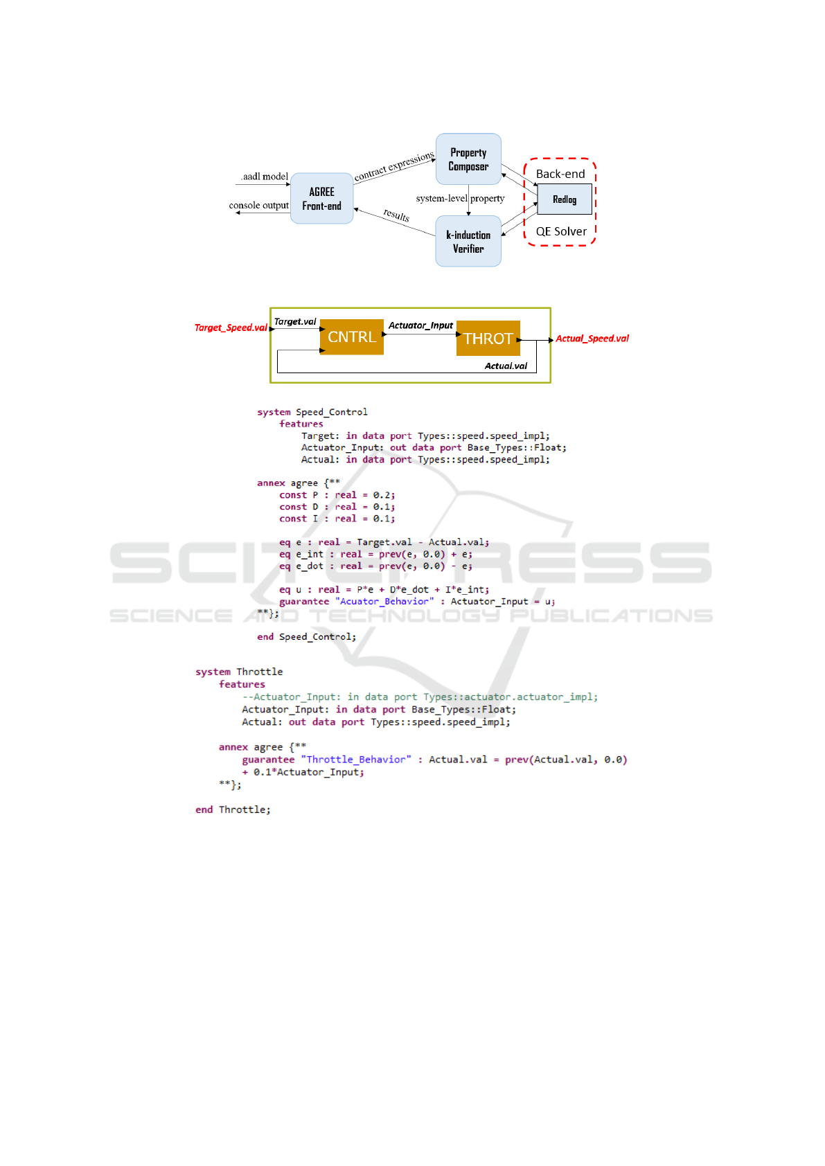
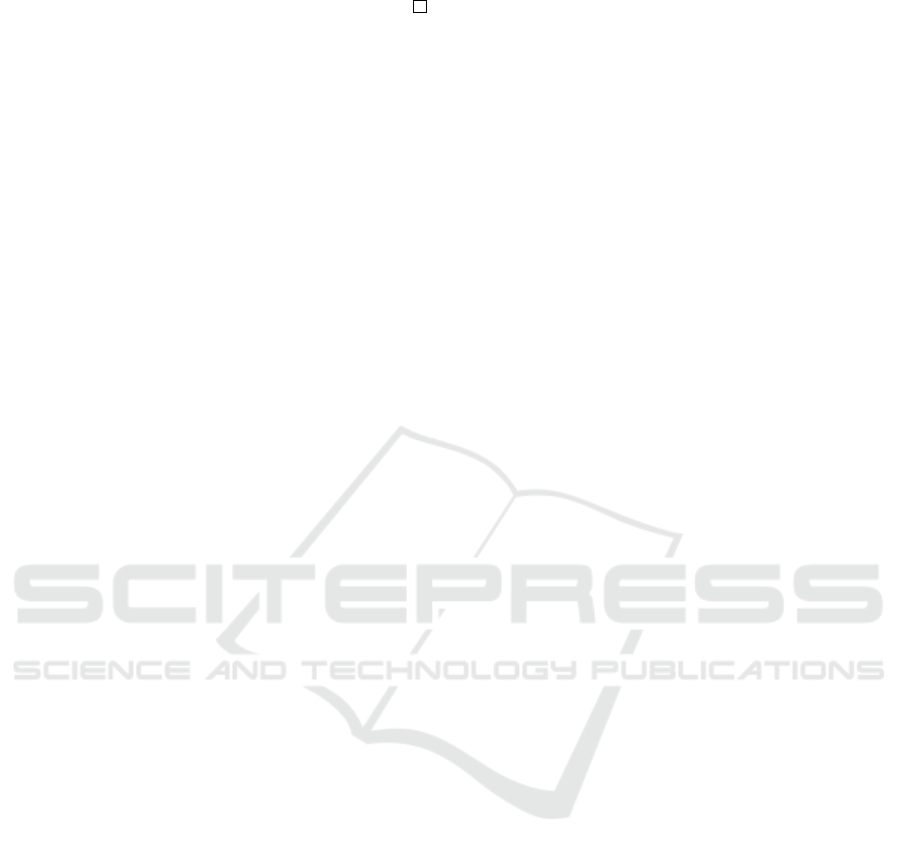
Figure 1: Architecture of ReLIC.

(a) A vehicle model and its components dynamics.

(b) Speciﬁcation of CNTRL component.

Figure 2: A vehicle model, modiﬁed from (Gacek et al., 2017).

tool ReLIC is shown in Fig. 1. It utilizes the front-end

infrastructure of the AGREE (Stewart et al., 2017) tool

for capturing and parsing the input AADL models that

describe the components, their connectivity, and their

properties, and also its output environment for pre-

senting the property composition and veriﬁcation re-

sults to the console. The “Property Composer” mod-

ule computes the upper bound for the system-level or-

der based on Theorem 3.1 and computes the strongest

system-level property based on Theorem 3.2. This

is then used by the “Induction Veriﬁer” module to

perform induction-based system-level veriﬁcation of

a postulated system property. Both these modules uti-

lize Redlog (red, 2015) as a back-end solver that sup-

ports quantiﬁer elimination.

To demonstrate our tool, we tested it on a vehi-

ICINCO 2019 - 16th International Conference on Informatics in Control, Automation and Robotics

538

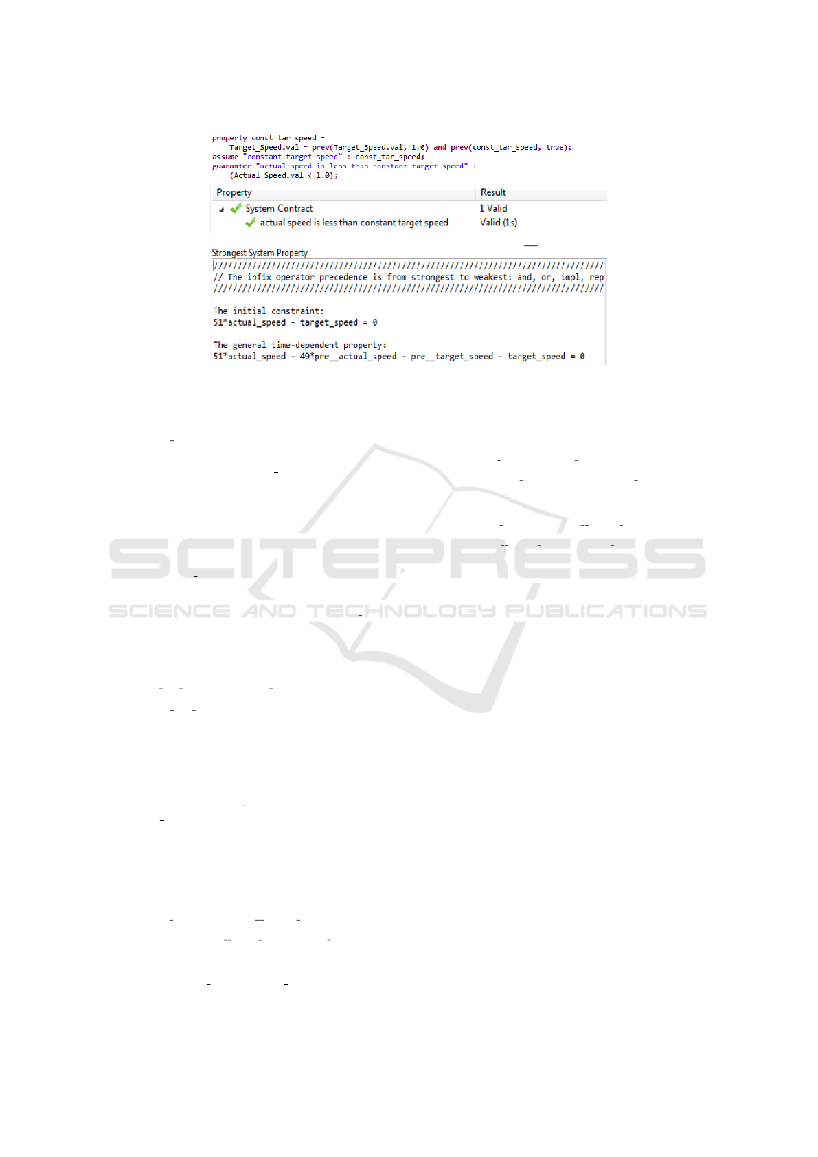
Figure 3: ReLIC veriﬁcation output on the vehicle model.

cle model as shown in Fig. 2a. The vehicle consists

of two components, namely, a PID control compo-

nent “Speed Control” (CNTRL) and a vehicle throt-

tle “Throttle” (THROT), within a feedback conﬁgura-

tion. The dynamics of “Speed Control” is speciﬁed

by a set of difference equations involving also cer-

tain state variables (Fig. 2b), whereas the dynamics of

“Throttle” is speciﬁed by a difference equation over

only its input and output variables (Fig. 2c).

There are three ﬁrst-order expressions in total,

namely,

e int = prev(e, 0.0) + e,

e dot = prev(e,0.0) − e, and

Actual.val = prev(Actual.val, 0.0) + 0.1 ∗ Actuator Input,

where prev(·) is the extended delay operator pre(·)

with the second argument denoting the initial value.

The postulated system property is

const tar speed ⇒ (Actual Speed.val < 1.0),

where const tar speed is a Boolean variable whose

truth indicates system target speed is set to a con-

stant value 1.0 (its deﬁning expression is given in

Fig. 3). The ReLIC inferred strongest system prop-

erty (based on (2) and (3)) contains the system-level

difference equation as well as the initial condition

over system input Target Speed.val and system out-

put Actual Speed.val. While the upper bound for the

composed system order is 3, it turns out that the sys-

tem input-output property order is only 1 due to the

inherent parallelism among the components, as also

computed by our approach (see the encoded expres-

sions below as well as the console output in Fig. 3):

51 ∗ actual speed − 49 ∗ pre actual speed

−pre target speed − target speed = 0,

with the initial condition:

51 ∗ actual speed −target speed = 0.

These are easily shown to imply the postulated

system property using induction, where the base step

is:

(51 ∗ actual speed −target speed = 0) ⇒



(target speed = 1) ⇒ (actual speed < 1)



and the inductive step is



(51 ∗ actual speed −49 ∗ pre actual speed

−pre target speed −target speed = 0)

∧(pre target speed = 1) ∧ (pre actual speed < 1)



⇒



(target speed = pre target speed) ⇒ (actual speed < 1)



Both the base and induction steps can be veri-

ﬁed to be true, again using quantiﬁer elimination, this

based on universal quantiﬁcation over the external

variables.

5 CONCLUSION

We introduced for a ﬁrst-time a property composi-

tion framework to support the composition of time-

dependent properties. This is a foundational step to-

wards compositional reasoning of systems possessing

bounded “memory”. The extension developed a new

procedure to determine the system order, given the

component orders, and used it to form the required

time-shifted replicas of the component properties and

their QE-based composition. We implemented our

compositional approach in our prototype tool ReLIC

that uses AADL for modeling system architecture and

component properties using the tool AGREE, and the

QE solver Redlog at the back-end for performing the

QE. The proof of a postulated system-level property

involves induction, which is also supported in our

ReLIC tool.

“ReLIC: Reduced Logic Inference for Composition” for Quantiﬁer Elimination based Compositional Reasoning

539

ACKNOWLEDGEMENTS

This work was partially supported by the National

Science Foundation under the grants NSF-CCF-

1331390, NSFECCS-1509420, NSF-IIP-1602089,

and a sabbatical support from the Air Force Research

Lab, Dayton, OH.

REFERENCES

(2012). Agree. Available from:

http://loonwerks.com/tools/agree.html.

(2015). redlog. Available from: http://www.redlog.eu/.

Emmi, M., Giannakopoulou, D., and P

areanu, C. S.

(2008). Assume-guarantee veriﬁcation for interface

automata. In International Symposium on Formal

Methods, pages 116–131. Springer.

Fadali, M. S. and Visioli, A. (2012). Digital control engi-

neering: analysis and design, chapter 7. State-Space

Representation. Academic Press.

Feiler, P. H., Gluch, D. P., and Hudak, J. J. (2006). The ar-

chitecture analysis & design language (aadl): An in-

troduction. Technical report, Carnegie-Mellon Univ

Pittsburgh PA Software Engineering Inst.

Gacek, A., Backes, J., Mike, W., Darren, C., and Jing, L.

(2017). Agree users guide, v0.9. Available from:

https://github.com/smaccm/smaccm/tree/master/ doc-

umentation/agree.

Gacek, A., Katis, A., Whalen, M. W., Backes, J., and Cofer,

D. (2015). Towards realizability checking of contracts

using theories. In NASA Formal Methods Symposium,

pages 173–187. Springer.

Kahsai, T. and Tinelli, C. (2011). Pkind: A parallel

k-induction based model checker. arXiv preprint

arXiv:1111.0372.

Kingston, D., Rasmussen, S., and Humphrey, L. (2016).

Automated uav tasks for search and surveillance. In

Control Applications (CCA), 2016 IEEE Conference

on, pages 1–8. IEEE.

Quinton, S. and Graf, S. (2008). Contract-based veriﬁcation

of hierarchical systems of components. In 2008 Sixth

IEEE International Conference on Software Engineer-

ing and Formal Methods, pages 377–381. IEEE.

Rasmussen, S., Kalyanam, K., and Kingston, D. (2016).

Field experiment of a fully autonomous multiple

uav/ugs intruder detection and monitoring system. In

Unmanned Aircraft Systems (ICUAS), 2016 Interna-

tional Conference on, pages 1293–1302. IEEE.

Ren, H., Clark, M., and Kumar, R. (2018). Integration of

quantiﬁer eliminator with model checker and compo-

sitional reasoner. In 2018 IEEE 14th International

Conference on Control and Automation (ICCA), pages

1070–1075. IEEE.

Ren, H., Clark, M. A., and Kumar, R. (2016). Integration of

quantiﬁer eliminator with model checker and compo-

sitional reasoner. In Air Force Research Laboratory’s

Safe & Secure Systems and Software Symposium.

Sheeran, M., Singh, S., and St

almarck, G. (2000). Check-

ing safety properties using induction and a sat-solver.

In International conference on formal methods in

computer-aided design, pages 127–144. Springer.

Stewart, D., Whalen, M. W., Cofer, D., and Heimdahl,

M. P. (2017). Architectural modeling and analysis for

safety engineering. In International Symposium on

Model-Based Safety and Assessment, pages 97–111.

Springer.

Tarski, A. (1998). A decision method for elementary al-

gebra and geometry. In Quantiﬁer elimination and

cylindrical algebraic decomposition, pages 24–84.

Springer.

ICINCO 2019 - 16th International Conference on Informatics in Control, Automation and Robotics

540