Approaches to Identify Relevant Process Variables in Injection Moulding

using Beta Regression and SVM

Shailesh Tripathi

, Sonja Strasser

, Christian Mittermayr

, Matthias Dehmer

and Herbert Jodlbauer

Production and Operations Management, University of Applied Sciences Upper Austria,

Wehrgrabengasse 1-3, Steyr, Austria

Greiner Packaging International GmbH, Greinerstrasse 70, 4550 Kremsmuenster, Austria

Keywords:

Injection Moulding, Beta Regression, SVM, Scrap Rate Prediction.

Abstract:

In this paper, we analyze data from an injection moulding process to identify key process variables which

inﬂuence the quality of the production output. The available data from the injection moulding machines

provide information about the run-time, setup parameters of the machines and the measurements of different

process variables through sensors. Additionally, we have data about the total output produced and the number

of scrap parts. In the ﬁrst step of the analysis, we preprocessed the data by combining the different sets of

data for a whole process. Then we extracted different features, which we used as input variables for modeling

the scrap rate. For the predictive modeling, we employed three different models, beta regression with the

backward selection, beta boosting with regularization and SVM regression with the radial kernel. All these

models provide a set of common key features which affect the scrap rates.

1 INTRODUCTION

Injection moulding is regarded as the most important

process to produce all kind of plastic products. Sim-

ply put, a melted polymer is injected into a mold cav-

ity, packed under pressure and cooled until it has so-

lidiﬁed enough. This is performed by an injection

molding machine using an appropriate injection mold.

During the whole process, the material, the mold de-

sign and the processing parameters of the injection

molding machine interact with each other and deter-

mine the quality of the plastic product (Chang and

Faison III, 2001). Since there is a huge variety of dif-

ferent processing parameters, the complexity of the

process creates a very high effort to keep the quality

characteristics under control. If the necessary quality

characteristics cannot be achieved, the parts are dis-

carded as scrap. Quality problems can be of differ-

ent types, such as shrinkage, warpage, color and burn

marks, surface texture quality, shape distortion, and

other aesthetic defects (Kashyap and Datta, 2015). In

a real world industrial production the scrap rate varies

in different proportions during the production pro-

cess. Variation in scrap rate depends on many process

variables which are machine speciﬁc, product speciﬁc

and material speciﬁc. The main objective of the qual-

ity control is to minimize the scrap rate during a pro-

duction process. The scraps rate can be higher due

to many uncontrolled process variables or their com-

binations. Most of the studies are based on control-

ling fewer variables through an experimental design

and then estimating the quality of the products. How-

ever, in our analysis, we analyze data from the real-

world injection molding process, which is recorded

during the production process through different sen-

sors which consist of > 75 process variables. The re-

sponse variable is the proportion of the scraps which

are produced during the injection molding process.

The input variables are the statistical features of dif-

ferent process variables recorded during the produc-

tion process. In this analysis, we do not distinguish

between different types of scrap.

The main objective of the paper is to identify key

features of process variables which affect the prod-

uct quality for the purpose of monitoring in future to

control the production quality of different products at

different machines.

This paper contributes to the application of ma-

chine learning methods to identify common key pro-

cess variables, which affect the quality of the produc-

tion output represented by the scrap rate. The Struc-

ture of the paper is as follows: In Section 2 we pro-

vide a brief overview of the related work. In Sec-

tion 3 we describe the details about the methods for

Tripathi, S., Strasser, S., Mittermayr, C., Dehmer, M. and Jodlbauer, H.

Approaches to Identify Relevant Process Variables in Injection Moulding using Beta Regression and SVM.

DOI: 10.5220/0007926502330242

In Proceedings of the 8th International Conference on Data Science, Technology and Applications (DATA 2019), pages 233-242

ISBN: 978-989-758-377-3

233

the data preprocessing, ﬁltering and normalization. In

Section 4, we present details about the modeling and

variable selection. In Section 5, we evaluate the pro-

posed methods on recorded data and compare the re-

sults. Additionally, we compare our approach with

two other methods (Ribeiro, 2005; Mao et al., 2018)

which utilize SVM and a deep-learning approach to

classify the product quality into different categories.

In the ﬁnal Section 6 we provide the concluding re-

marks about the results and our analysis.

2 LITERATURE REVIEW

A large number of studies have been performed for

the quality optimization of the injection molding pro-

cess. Many studies of quality optimization are based

on Taguchi experimentation with a fewer number

of key process variables, which are responsible for

the product quality (Taguchi et al., 1987; Taguchi

et al., 1989; Unal and Dean, 1991; Chang and Fai-

son III, 2001; Barghash and Alkaabneh, 2014; Pack-

ianather et al., 2015; Chen et al., 2016; Oliaei et al.,

2016; Jahan and El-Mounayri, 2016). Several com-

putational approaches have been studied to optimize

product quality. These computational techniques are

based on gradient-based approaches, evolutionary al-

gorithms and mixed approaches utilizing gradient-

based approaches with evolutionary algorithms (Yin

et al., 2011b; Zafo

snik et al., 2015; Oliaei et al., 2016;

Yin et al., 2011a; Chen et al., 2016). Reviews of the

frameworks for the optimization of injection mould-

ing methods are described by (Kashyap and Datta,

2015; Dang, 2014; Singh and Verma, 2017; Fernan-

des et al., 2018).

3 METHODOLOGY

In this section, we provide a brief overview of the

methods we used for preprocessing, feature extrac-

tion, and the regression models. First, we describe the

available data for our analysis and the major prepro-

cessing steps. After splitting the data into different

production lots (segments), we extract relevant fea-

tures for the subsequent regression models. The aim

is to train prediction models for the scrap rates to get

information about the various setup parameters and

process variables which have the highest impact on

the scrap rates.

3.1 Data Collection

The data collection process starts by collecting raw

data from 33 injection molding machines which are

recorded into different ﬁles during a production pro-

cess. Additionally, we use data from the enterprise

resource planning (ERP) system. The relevant ﬁles

for our analysis are the production ﬁles, the process

ﬁles and an export ﬁle from the ERP system, which

have the following information:

Production ﬁle: provides time stamps, cycle

counter, tool-name, raw-material information,

cavities and set cycle time.

Process data: provides time stamps, cycle counter,

set cycle time and > 75 different process variables

such as actual cycle time, temperature, pressure,

volumes, positions, rotational speed, etc.

ERP data: provides the order number, material

number, number of produced parts and number of

scrap parts

The production and process data ﬁles contain data

from a certain time period where multiple product

types are produced. However, in the process data it-

self, there is no information about the product types.

So we used the production data and the ERP data to

split the process data into different segments accord-

ing to the product type and order number these differ-

ent segments based on product types and order num-

bers are described as process segments. Each pro-

cess segment contains information about > 75 differ-

ent process variables for the production process of a

product type between the start time and the end time

of production order. So the segment data ﬁle is a

multivariate time series data ﬁle, where columns are

the process variables and the rows are their respective

measures at different time points.

Relevant meta information about each production

order is collected in a separate master data ﬁle, includ-

ing start and end time of production, order number,

machine number, raw material number, total produc-

tion output in units and the number of scrap parts in

units.

3.2 Feature Extraction

For our analysis we extracted 6 statistical features of

each process variable due to following reasons:

– The values recorded for different process vari-

ables are not recorded for ﬁxed time intervals and

not all process variables are recorded at the same

time stamp.

DATA 2019 - 8th International Conference on Data Science, Technology and Applications

234

– For the predictive modelling we want to make our

results interpretable for the machine operators so

that they can tune the key process variables appro-

priately.

Let us assume that X is a process variable which

have values X = {x

,...x

} between time point

and time point t

. We extract common statistical

features: mean, standard deviation, maximum, min-

imum, M

(X) and M

(X) in each process segment

data ﬁle for each process variable. These statistical

features are described in Appendix section 6.1. Thus

for each process variables, we have six features. We

store all the extracted features for each process seg-

ment data ﬁle in a data set, D.

3.3 Scrap Rate

The extracted features are the predictor variables for

the prediction of the scrap rate. We add the scrap rate

as the response variable in the data ﬁle D and calculate

it, for each process segment p

, from the masterdata

ﬁle we extract the scraps samples and scaled the value

of the scrap between 0 and 1, r

∈ (0,1). The r

the new rescaled scrap rate for each process segment.

3.4 Data Filtering

For our analysis, we ﬁlter out those process segments

which are running longer than 120 hours and shorter

than 20 minutes. This information is extracted from

the master data ﬁle. After this ﬁltering step, D con-

tains 1996 observations and 558 features.

Since we collected data from different injection

molding machines, we do not have the same set of

process variables for each machine and therefore de-

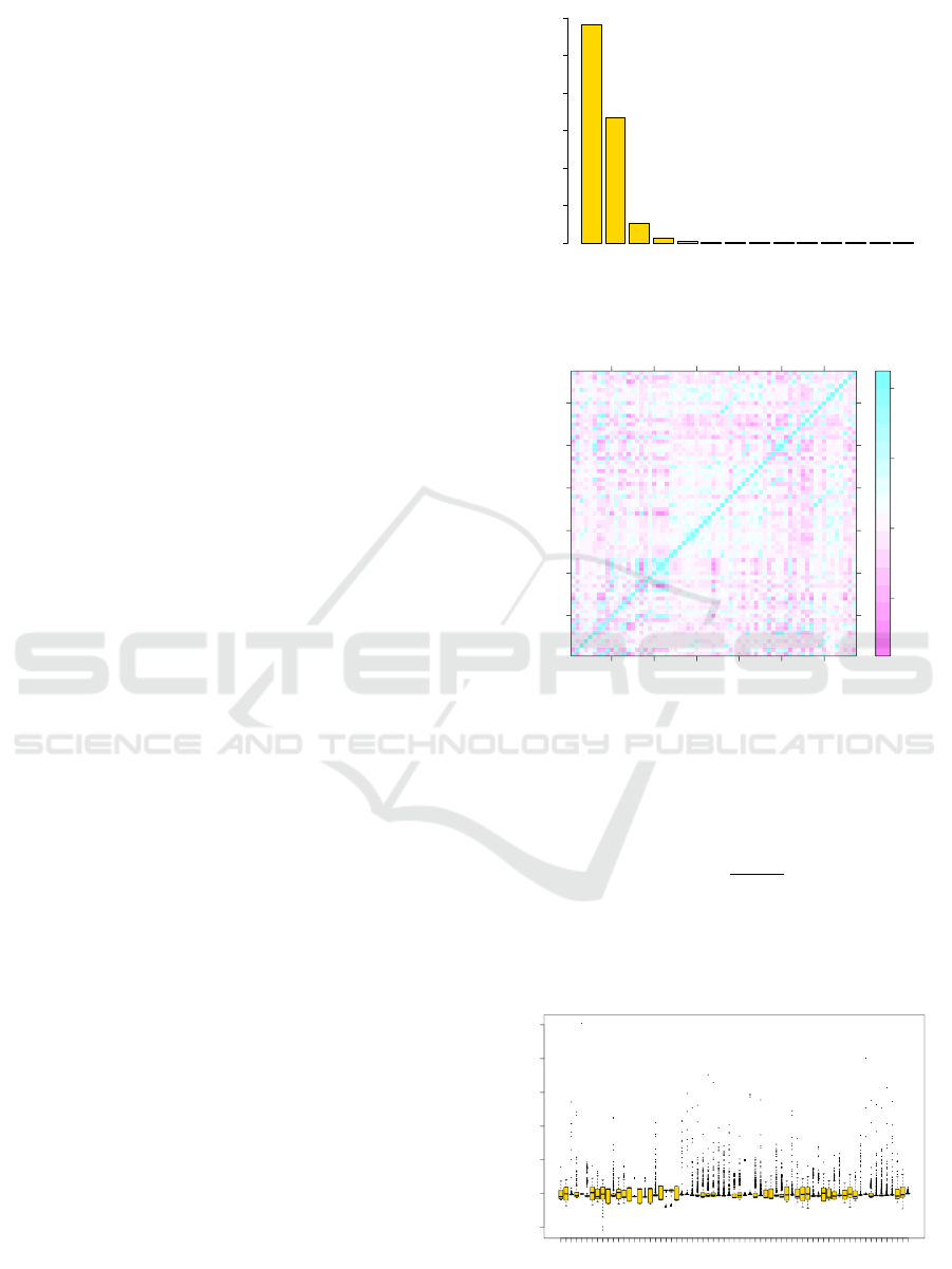
viating features for the process segments. In order to

ﬁnd a common set of features, we analyzed the fre-

quency of observations of the extracted features. The

result is shown in Figure 1. Then we select those fea-

tures which appear in common at least in ≥ 600 obser-

vations. Thus we obtained 639 common observations

for 327 features.

In the next step of ﬁltering, we ﬁlter out highly

correlated variables which have a high correlation of

ρ > .95 with any of the other feature variables. Our

approach to ﬁlter out such variables is described in

Algorithm 3 in Appendix section 6.1. After this step,

we have a |L| = 66 features. The correlation between

these different features is shown in Figure 2

3.5 Data Normalization

We normalized each feature independently as follows:

Suppose a feature V

= {v

,...,v

} has n sam-

663

180

843

633

651

581

564

521

520

411

380

235

156

# features

100

150

200

250

300

# Observations

Figure 1: The Frequency of Observations of Different Fea-

ture Variables.

extracted features

10 20 30 40 50 60

−0.5

0.0

0.5

1.0

Figure 2: Correlation between Different Features of Process

Variables after Filtering.

ples. We convert samples of each features into stan-

dard scores as follows:

normalized

−

. (1)

The distributions of normalized features are shown in

Figure 3. These features in the Figure 3 are ordered

as per the Table 7 in the Appendix.

1 3 5 7 9 12 15 18 21 24 27 30 33 36 39 42 45 48 51 54 57 60 63 66

−5 0 5 10 15 20 25

features

distribution of normalized data

Figure 3: Distributions of Normalized Features.

Approaches to Identify Relevant Process Variables in Injection Moulding using Beta Regression and SVM

235

4 MODEL AND VARIABLE

SELECTION

For the selection of the most important features from

our data, we applied three different models, which are

beta regression with a backward selection procedure,

beta boosting approach with regularization and SVM

regression with the radial kernel. The details of the

methods are provided below.

4.1 Beta Regression Model

This model is proposed by Ferrari and Cribari-Neto

(Ferrari and Cribari-Neto, 2004). The beta regression

model is used to predict rates and proportions where

the prediction variables y ∈ (0, 1). The underlying as-

sumption of the beta regression model is that the re-

sponse variable is beta distributed. In such cases, the

linear models are not useful for two reasons:

– The model parameters are interepreted with re-

spect to the transformed response ˜y = log(y/(1 −

y)) and not with the real response y.

– The heteroskedastic nature of the data.

The beta distribution in terms of µ and φ is ex-

pressed as follows:

f (y; µ,φ) =

Γ(φ)

Γ(µφ)Γ((1 − µ)φ)

µφ−1

(1 − y)

(1−µ)(φ−1)

(2)

where, µ = p/(p + q) and φ = p + q (p,q > 0 real pa-

rameters of the distribution, Γ(x) Gamma function).

The expected value and variance are E(y) = µ and

Var(y) = µ(1 − µ)/(1 + φ). φ is a precision param-

eter.

In the beta regression model, we suppose to have

,...,y

random samples where y

∼ B(µ

,φ), i =

1,2,...,n. The beta regression model is described as

follows:

g(µ

) = x

β (3)

with a link function g(x), which can be logit, probit

or log − log link. The expected value µ

is described

as follows:

= g

−1

β) (4)

In order to remove the bias of maximum likeli-

hood estimates of parameters an extension by intro-

ducing a regression structure on the precision param-

eter φ can be used (Simas et al., 2010):

(µ

) = x

β (5)

(φ

) = z

γ (6)

The logit, probit and log-log link function are de-

ﬁned as follows:

logit: g(µ) = log(

1 − µ

) (7)

probit: g(µ) = Φ

−1

(µ) (8)

The Φ(.) is a standard normal distribution function

log-log: g(µ) = −log(−log(µ)) (9)

The improved beta regression model allows non

linear predictors for g

(µ

) and g

(φ

) and also gives

the bias corrected estimate of maximum likelihood.

For our data analysis we used the betareg R package

(Cribari-Neto and Zeileis, 2010).

4.2 Beta Boosting Model

The boosting approach of beta regression model

(Schmid et al., 2013) is based on generalized addi-

tive models for location, scale and shape (GAMLSS)

approach (Thomas et al., 2018; Buehlmann and

Hothorn, 2007; Rigby and Stasinopoulos, 2005). The

beta boosting model uses the gamboostLSS boosting

algorithm for the variable selection (Hofner et al.,

2016). The brief explanation of beta boosting regres-

sion is described in Algorithm 1.

Algorithm 1: Betaboosting Algorithm.

B = 10000

Set iterator itr = 1

Set the initial parameter, β = 0 and γ = 0 (values

for g

(µ) and g

(φ)).

repeat

Keep the γ ﬁxed and select predictor variables

by considering the mean model described in Equa-

tion 5.

Update β

coefﬁcient for which the predictor

variable, X

, improves the beta log likelihood es-

timate.

Keep β ﬁxed and select predictor variables con-

sidering precision model described in Equation 6.

Update γ

coefﬁcient for which the predictor

variable, Z

, improves the beta log likelihood es-

timate.

itr = itr +1

until itr = B

4.3 SVM Regression

The support vector regression is based on the support

vector machine concept (Drucker et al., 1996; Vapnik,

1995). In SVM regression the input data is mapped

DATA 2019 - 8th International Conference on Data Science, Technology and Applications

236

to the the high dimensional feature space using non-

linear mapping, which is described as follows: Let

f : X → R

f (x) =< w,φ(x) > +b (10)

The φ(x) is a high dimensional feature space. By us-

ing a kernel trick, a kernel function can be used to

calculate the inner product in feature space, which is

described as follows:

f (x) =

∑

i=1

k(x

,x) + b (11)

Where α = (K + λI)

−1

y. In our regression model we

use the radial kernel function, which is described as

follows:

k(x, x

) = exp(

||x − x

2σ

) (12)

4.4 Backward Feature Selection for

Beta Regression

For the backward feature selection in beta regres-

sion model, we followed a bootstrapped approach

where we generate 500 bootstrapped datasets, D =

...,D

B=500

. For each bootstrap data, we model

the beta regression model M

, where b = 1,2,...,500.

We estimate the parameters and compute the weight

of each parameter in the model as follows:

∑

b=1

I(p(M

)) <= α) (13)

where i = 1,2,...n. The function p(M

) returns the

p-value for parameter i from model M

and α is the

deﬁned signiﬁcance level. We discard the variable

which is least weighted and repeat the analysis un-

til the weights of remaining variables are greater then

a certain threshold. In our analysis we set this thresh-

old, thr = 0.9. The detailed description of feature se-

lection is shown in Algorithm 2.

4.5 Feature Selection in SVM

Regression

For the feature selection in SVM regression, we ap-

plied the recursive feature elimination (RFE) method

to ﬁnd the most important features which predict

the outcome with higher accuracy. We applied the

RFE algorithm with resampling, which iteratively re-

jects the weakest predictor variable. In our anal-

ysis, for each iteration we ﬁrst tune hyperparame-

ters σ = {.01,.05, .1 . . . , 1} and box constraint C =

{0.01,.1,.5,1,2,4,8,...,512,1024} and then we per-

form the RFE on the best model by tuning hyperpa-

rameters.

Algorithm 2: Backward Selection using Beta Regression.

Set B = 500

Set thr = 0.9

Set α = 0.05

Set D is the training dataset of n × m dimension.

repeat

,...,D

500

are 500 bootstrapped datasets.

...M

500

beta regression models for the

bootstrapped datasets.

Let p(M

) be a function that returns the p −

value of the parameter i in the model M

A is a vector of size m.

for t = 1 to m do

k =

∑

b=1

I(p(M

) <= α)

A[t] = k/B

end for

Let i = r (A)  returns the lowest rank index of

parameter

if A[i] < thr then

D = D

 Discard the variable i in data D

else

i = NULL

until i = NULL

return A  index of selected parameters.

5 RESULTS

5.1 Betaregression Model

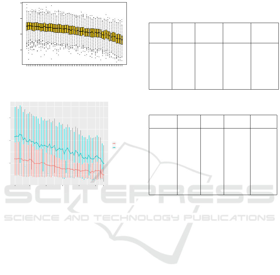
By applying Algorithm 2, we obtained eight impor-

tant features which are signiﬁcant consistently in the

backward selection. In Figure 4 we show the boxplots

of R

measures as we discard the weakest variables in

each step. The x-axis displays the number of variables

in different models, and the y-axis shows the distribu-

tion of R

values from different models built on the

bootstrapped datasets. The R

results show gradually

decrease as we discard a variable in each step. The av-

erage R-square is

= 0.562 with ﬁnally eight vari-

ables. Figure 5 visualizes the validation errors and

test errors. The validation and test errors decrease as

we discard the weakest variable. The error is lowest

when there are only eight variables in the model.

5.2 Betaboosting Model

For the betaboosting model we analyze the

same training data for different step lengths

S = {.001,.01, .05, , 0.1, 0.2, 0.5, 1} with 10,000

iterations. Table 1 shows the results for each step

length. As performance measures R

and the RMSE

are calculated. The beta boosting model detects

Approaches to Identify Relevant Process Variables in Injection Moulding using Beta Regression and SVM

237

62 58 54 50 46 42 38 34 30 26 22 18 14 10

0.5 0.6 0.7 0.8

# number of variables

− (r − squared)

Figure 4: Distribution of R

Measures for Different Beta

Regression Models using Bootstrapped Samples.

0.09

0.11

0.13

62 53 43 33 23 13 8

variables

error

test error

validation error

Figure 5: RMSE of Different Beta regression Models using

Bootstrapped Samples.

different number of features for µ and φ which are

shown in Table 1. The best model have higher

= 0.616 measure compare to the beta regression

model.

5.3 SVM Regression Model

In the ﬁrst step of the analysis, we train our model

with SVM regression using all the feature variables.

This model provides improved accuracy in terms of

measure and RMSE. The higher accuracy indi-

cates a non-linear relationship between the scrap rate

and the input feature variables. We further applied

the RFE algorithm and tuned the model with ten-fold

cross-validation with various combinations of hyper-

parameters. The results of the best performing models

are shown in Table 2. The SVM model recognizes 42

feature variables as important variables.

5.4 Comparison of Models

The three different models identify a different number

of features as important predictors for the scrap rate.

The simplest beta regression model predicts 8 feature

Table 1: R

measure and number of signiﬁcant features for

µ and φ in Betaboosting regression models using different

step lengths.

Step

length

# of fea-

tures for

# of fea-

tures for

RMSE

0.001 0.51 11 7 0.103

0.01 0.58 27 17 0.0885

0.05 0.605 40 36 0.0857

0.1 0.616 45 54 0.0846

0.2 0.607 42 36 0.0856

0.5 0.613 27 39 0.0847

1.0 0.597 14 19 0.090

Table 2: The results of best performing SVM models with

different combinations of hyper-parameters.

SVM

Models

Sigma C Rsquared RMSE

1 0.050 4 0.675 0.0758

2 0.010 32 0.671 0.0757

3 0.010 16 0.667 0.0774

4 0.010 64 0.657 0.0775

5 0.100 4 0.655 0.0778

6 0.050 16 0.654 0.0777

7 0.005 64 0.653 0.0790

8 0.050 2 0.649 0.0809

9 0.100 2 0.646 0.0798

10 0.005 32 0.646 0.0808

variables; the beta boosting model predicts 45 feature

variables and SVM regression detects 42 important

feature variables. 6 feature variables are common in

all three models, 7 feature variables are common in

the beta regression model, and the SVM model. The

31 feature variables are common in the beta boost-

ing model and SVM regression. The common 6 vari-

ables, which are present all three models, are shown

in Table 3. Apart from the common features, different

features are ranked high by the beta boosting model

and SVM model. These top features are shown in

Table 5 for each approach. The reason for different

feature weights depends on the underlying assump-

tions of different models; therefore different features

are weighted high by different models.

We further test these three models on the test-

ing data, which consists of 160 testing samples, the

RMSE of the different models are shown in Table

4. The predicted scrap rates for the testing data are

shown in Figure 6 for each applied model. By ana-

lyzing these three models, we found that up to 65%

of the variance in scrap can be described by at least ∼

42 features of process variables as shown by the SVM

model. However, a large percentage of variance in the

output is described by 8 feature variables resulting in

the beta regression model.

DATA 2019 - 8th International Conference on Data Science, Technology and Applications

238

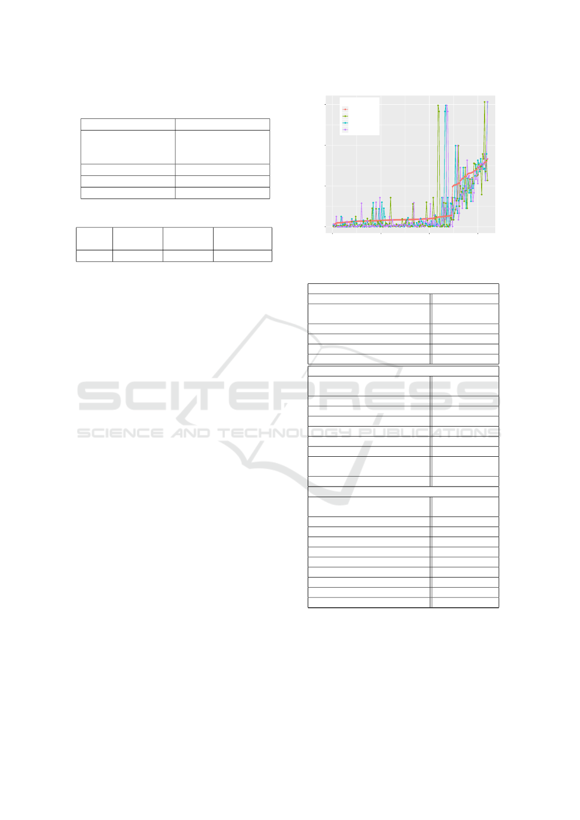
Table 3: Common Process Variables and their most Impor-

tant Features.

Process variables Features

Screw volume (end

of holding-pressure

phase)

X,S(X ),M

(x)

Torque peak value max(x)

Temperature zone 7 max(x)

Temperature zone 11 max(x)

Table 4: RMSE on Testing Data for Different Models.

Models Beta Re-

gression

Beta

Boosting

SVM

Regression

RMSE 0.0792 0.0793 0.0764

The nonlinear models do not add more value to

the results, which leads to the conclusion that a small

number of variables are linearly related to the scrap

rate. Also, the processed data do not explain the re-

maining variance in the data. The RMSE of the test-

ing data suggests that the SV M model leads to the

lowest prediction error. However, the testing error

of the Beta regression model is only slightly higher

than the SV M model. The testing data show a higher

variance for some of the process segments, and this is

common in all models for different scrap rates. The

high variance in the prediction when scrap is higher

can be due to some technical faults, which are unno-

ticed or not recorded. Similarly, an unexplained vari-

ance in the scrap rate prediction by predictive models

also have a dependency on other features such as ma-

terial type, product shape, and other external factors.

5.5 Comparison with Related Studies

We compare our approach with two other approaches

shown in Table 6. The ﬁrst difference is that the

data in these two approaches is generated from an

experimental design by controlling fewer (≤ 6) pro-

cess variables on a single machine. The data is gen-

erated by controlling fewer process variables of dif-

ferent categories of products quality. These meth-

ods utilize machine learning approaches for the clas-

siﬁcation of product quality using SVM and deep-

learning approaches. In our analysis, we predict the

scrap rate as an output of the whole production pro-

cess by using statistical features of process variables,

which is a high dimensional data of ∼ 65 feature vari-

ables. Also, we do not differentiate between different

types of scraps. The results in both the studies pre-

dict scrap class with higher accuracy, but they are not

directly comparable with our results due to the nature

of the data and the output. However, our models pre-

r(p

) - predicted

0.0

0.2

0.4

0.6

0 50 100 150

testing data index (ordered)

Models

Testing data

Beta boosting

Beta regression

SVM regression

Figure 6: Predicted r

by different models on testing data.

Table 5: Top Process Variables ranked by Different Models.

Beta Regression

Process variables Features

Screw volume (end of holding-

pressure phase)

(X),S(X),

Discharge end 1 max(X),M

(X)

Torque peak value max(X)

Temperature zone 7 max(X)

Temperature zone 11 max(X)

Beta boosting

Screw volume (end of holding-

pressure phase)

S(X)

Torque peak value max(X),min(X )

Temperature zone 6 max(X)

Shot volume max(X)

discharge end 1 S(X)

Integral monitoring micrograph max(X)

Temperature zone 7 M

(X)

Hydraulic pressure at switch

point

(X)

Idle time before cycle start M

(X)

SVM Regression

Screw volume (end of holding-

pressure phase)

S(X)

Shot volume max(X)

Temperature zone 7 min(X)

Temperature zone 8 max(X)

Torque peak value max(X),min(X )

Actual value pressure pump M

(X)

Cycle time M

(X),max(X )

Actual value injection time min(X)

Idle time before cycle start M

(X)

Temperature zone 6 max(X)

dict some common features which show importance

in previous studies such as cycle time, screw volume,

torque, different temperature zones and pressure pa-

rameters (Singh and Verma, 2017).

Approaches to Identify Relevant Process Variables in Injection Moulding using Beta Regression and SVM

239

6 CONCLUSIONS

In this paper, we analyzed production data from an in-

jection molding process, which contains ∼ 70 process

variables from different machines. We start our analy-

sis by preprocessing, cleaning and ﬁltering of relevant

information from the raw data. We extracted impor-

tant statistical features of different process variables.

After ﬁltering using Algorithm 3, we selected 66 of

them. These 66 features are used for scrap rate pre-

diction using linear and non-linear models. We ﬁrst

applied the beta regression model with a backward

feature selection method, which provides a signiﬁ-

cant estimate of the scrap rate. We extend it for the

non-linear models to explore the non-linear relation-

ship between the scrap rate and the feature variables.

The non-linear models provide a slight improvement

in prediction, but due to a large number of selected

features, the models become more complex.

In this analysis, we try to understand more gen-

eral, which feature variables affect the quality of the

production process. A simple beta regression model

provides a good prediction for the scrap rate with

fewer feature variables than the non-linear models.

However, the unexplained variance of the response

variable also depends on many other aspects of the

product such as the material type, size, volume and

many other product speciﬁc features, which are not

the part of the analysis. Additionally, there are many

machine-speciﬁc features which have been discarded

in our prepossessing due to not having enough sam-

ples and variance. The product and machine spe-

ciﬁc features which are absent in the model can be

the reason for the unexplained variance of the predic-

tive models. The features of the process variables,

identiﬁed by different methods, are general features

which affect the product quality of different product

types. Particular attention should be paid to tuning of

these process parameters for a better production qual-

ity. However, the product quality also depends on ma-

terial types, volume and size, and other product and

machine speciﬁc parameters. Therefore, in our future

work, for the product-speciﬁc quality control, we will

look into the data in more details by exploring more

product and machine speciﬁc details which affect the

production output. We want to extend our data mod-

eling for the different type of product speciﬁc quality

measures.

The Authors have no competing interest.

Table 6: Comparison of three different approaches for the

prediction of product quality.

Methods

proposed by

Objective and

Methodology

Data genera-

tion

Input variables and Out-

put

(Ribeiro,

2005)

Product qual-

ity prediction

using Sup-

port vector

machine

based ap-

proaches

by tuning

different

hyperparam-

eters for error

classiﬁcation

Data is gen-

erated by an

experimental

set up on

Demag injec-

tion molding

machine with

Hostacom

DM2 T06

polymer and

with mold

DN502

Input variables: cycle

time, dosage time,

injection time, cushion,

peak melt temperature

and, ram velocity

Output: Product quality

of different categories

which are Streak,

Strains, Burn marks,

Edges, Unﬁlled parts

and Warped parts

(Mao et al.,

2018)

Feature

learning

and process

monitoring

using Deep

learning

approach of

Convolution-

deconvolution

auto encoder

Data is gen-

erated by an

experimental

set up on

on a JSW

J110ADC-

180H electric

injection

molding

machine by

tuning differ-

ent process

conditions

to generate

different

batches

of good

and faulty

quality.

The data is in the form

of 4D input Tensor,

χ(B × V × T × C),

where, V is the number

of variables, B is the

batch size of a product

quality class, C is the

number of feature chan-

nels, and T is the set

of time instances where

the values of different

process variables are

measured. V={screw

displacement, injection

pressure, cavity pres-

sure }

Output: Different

conditions of product

quality

Our ap-

proach

Identiﬁcation

of key pro-

cess variables

which affect

the prod-

uct quality

(scrap rate)

using Beta

regression,

beta boosting

and SVM

regression

methods

Observational

data from

real time

production

of different

products of

shape, size

and material

type pro-

duced by

33 different

machines in

the company.

65 Statistical features

extracted from different

process variables

Output: Scrap rate

which is the proportion

of total scraps and the

total output produced.

ACKNOWLEDGEMENTS

This paper was funded through the project ADAPT by

the Government of Upper Austria in their programme

”Innovative Upper Austria 2020”.

REFERENCES

Barghash, M. A. and Alkaabneh, F. A. (2014). Shrinkage

and warpage detailed analysis and optimization for

DATA 2019 - 8th International Conference on Data Science, Technology and Applications

240

the injection molding process using multistage exper-

imental design. Quality Engineering, 26(3):319–334.

Buehlmann, P. and Hothorn, T. (2007). Boosting algo-

rithms: Regularization, prediction and model ﬁtting.

Statist. Sci., 22(4):477–505.

Chang, T. C. and Faison III, E. (2001). Shrinkage behavior

and optimization of injection molded parts studied by

the taguchi method. Polymer Engineering & Science,

41(5):703–710.

Chen, W.-C., Nguyen, M.-H., Chiu, W.-H., Chen, T.-N.,

and Tai, P.-H. (2016). Optimization of the plastic

injection molding process using the taguchi method,

rsm, and hybrid ga-pso. The International Journal

of Advanced Manufacturing Technology, 83(9):1873–

1886.

Cribari-Neto, F. and Zeileis, A. (2010). Beta regression in r.

Journal of Statistical Software, Articles, 34(2):1–24.

Dang, X.-P. (2014). General frameworks for optimization

of plastic injection molding process parameters. Sim-

ulation Modelling Practice and Theory, 41:15 – 27.

Drucker, H., Burges, C. J. C., Kaufman, L., Smola, A.,

and Vapnik, V. (1996). Support vector regression ma-

chines. In Proceedings of the 9th International Con-

ference on Neural Information Processing Systems,

NIPS’96, pages 155–161, Cambridge, MA, USA.

MIT Press.

Fernandes, C., Pontes, A. J., Viana, J. C., and Gaspar-

Cunha, A. (2018). Modeling and optimization of the

injection-molding process: A review. Advances in

Polymer Technology, 37(2):429–449.

Ferrari, S. and Cribari-Neto, F. (2004). Beta regression for

modelling rates and proportions. Journal of Applied

Statistics, 31(7):799–815.

Hofner, B., Mayr, A., and Schmid, M. (2016). gamboostlss:

An r package for model building and variable selec-

tion in the gamlss framework. Journal of Statistical

Software, Articles, 74(1):1–31.

Jahan, S. A. and El-Mounayri, H. (2016). Optimal con-

formal cooling channels in 3d printed dies for plastic

injection molding. Procedia Manufacturing, 5:888

– 900. 44th North American Manufacturing Re-

search Conference, NAMRC 44, June 27-July 1,

2016, Blacksburg, Virginia, United States.

Kashyap, S. and Datta, D. (2015). Process parameter opti-

mization of plastic injection molding: a review. Inter-

national Journal of Plastics Technology, 19(1):1–18.

Mao, T., Zhang, Y., Ruan, Y., Gao, H., Zhou, H., and Li, D.

(2018). Feature learning and process monitoring of

injection molding using convolution-deconvolution

auto encoders. Computers & Chemical Engineering,

118:77 – 90.

Oliaei, E., Heidari, B. S., Davachi, S. M., Bahrami, M.,

Davoodi, S., Hejazi, I., and Seyﬁ, J. (2016). Warpage

and shrinkage optimization of injection-molded plas-

tic spoon parts for biodegradable polymers using

taguchi, anova and artiﬁcial neural network meth-

ods. Journal of Materials Science & Technology,

32(8):710 – 720.

Packianather, M., Grifﬁths, C., and Kadir, W. (2015). Micro

injection moulding process parameter tuning. Proce-

dia CIRP, 33:400 – 405. 9th CIRP Conference on

Intelligent Computation in Manufacturing Engineer-

ing - CIRP ICME ’14.

Ribeiro, B. (2005). Support vector machines for qual-

ity monitoring in a plastic injection molding process.

IEEE Transactions on Systems, Man, and Cybernet-

ics, Part C (Applications and Reviews), 35(3):401–

410.

Rigby, R. A. and Stasinopoulos, D. M. (2005). Generalized

additive models for location, scale and shape. Jour-

nal of the Royal Statistical Society. Series C (Applied

Statistics), 54(3):507–554.

Schmid, M., Wickler, F., Maloney, K. O., Mitchell, R.,

Fenske, N., and Mayr, A. (2013). Boosted beta re-

gression. PLOS ONE, 8(4):1–15.

Simas, A. B., Barreto-Souza, W., and Rocha, A. V. (2010).

Improved estimators for a general class of beta regres-

sion models. Computational Statistics & Data Anal-

ysis, 54(2):348 – 366.

Singh, G. and Verma, A. (2017). A brief review on in-

jection moulding manufacturing process. Materials

Today: Proceedings, 4(2, Part A):1423 – 1433. 5th

International Conference of Materials Processing and

Characterization (ICMPC 2016).

Taguchi, G., Elsayed, E., and Hsiang, T. (1989). Qual-

ity engineering in production systems. McGraw-Hill

series in industrial engineering and management sci-

ence. McGraw-Hill.

Taguchi, G., Konishi, S., Konishi, S., and Institute, A. S.

(1987). Orthogonal Arrays and Linear Graphs: Tools

for Quality Engineering. Taguchi methods. American

Supplier Institute.

Thomas, J., Mayr, A., Bischl, B., Schmid, M., Smith, A.,

and Hofner, B. (2018). Gradient boosting for distri-

butional regression: faster tuning and improved vari-

able selection via noncyclical updates. Statistics and

Computing, 28(3):673–687.

Unal, R. and Dean, E. B. (1991). Taguchi approach to de-

sign optimization for quality and cost : An overview.

Vapnik, V. N. (1995). The Nature of Statistical Learning

Theory. Springer-Verlag, Berlin, Heidelberg.

Yin, F., Mao, H., and Hua, L. (2011a). A hybrid of back

propagation neural network and genetic algorithm for

optimization of injection molding process parame-

ters. Materials & Design, 32(6):3457 – 3464.

Yin, F., Mao, H., Hua, L., Guo, W., and Shu, M.

(2011b). Back propagation neural network model-

ing for warpage prediction and optimization of plas-

tic products during injection molding. Materials &

Design, 32(4):1844 – 1850.

Zafo

snik, B., Bo

c, U., and Florjani

c, B. (2015). Mod-

elling of an analytical equation for predicting maxi-

mum stress in an injections moulded undercut geome-

try during ejection. International Journal of Precision

Engineering and Manufacturing, 16(12):2499–2507.

Approaches to Identify Relevant Process Variables in Injection Moulding using Beta Regression and SVM

241

APPENDIX

Statistical Features

X =

+ x

+ · ·· + x

(14)

S(X) =

∑

i=1

−

n − 1

(15)

min(X) = min(x

,. ..x

) (16)

max(X) = max(x

,. ..x

) (17)

(X) =

max(X) − min(X)

(18)

(X) =

max(X)

(19)

Data Filtering Algorithm

Algorithm 3: Filtering out the features which have correla-

tion, ρ ≥ .95.

Initialize:

R is a p × p sample correlation matrix

V = {V

,...,V

} is a ordered set of features

based on the number of other features with which

it has correlation, ρ ≥ .95, which is calculated as

follows.

a(V

) =

(p−1)

∑

k=1

I(ρ(i, k

) ≥ 0.95)

V = {V

,...,V

}, is ordered by

a(V

) > a(V

) > ··· > a(V

)

L is an empty vector.

cnt = 1

repeat

L[cnt] = V

⊂ V is a set of features with which

R[V

] ≥= .95

Update V : V = V \V

cnt = cnt + 1

until V is empty

return L

Features After Data Filtering

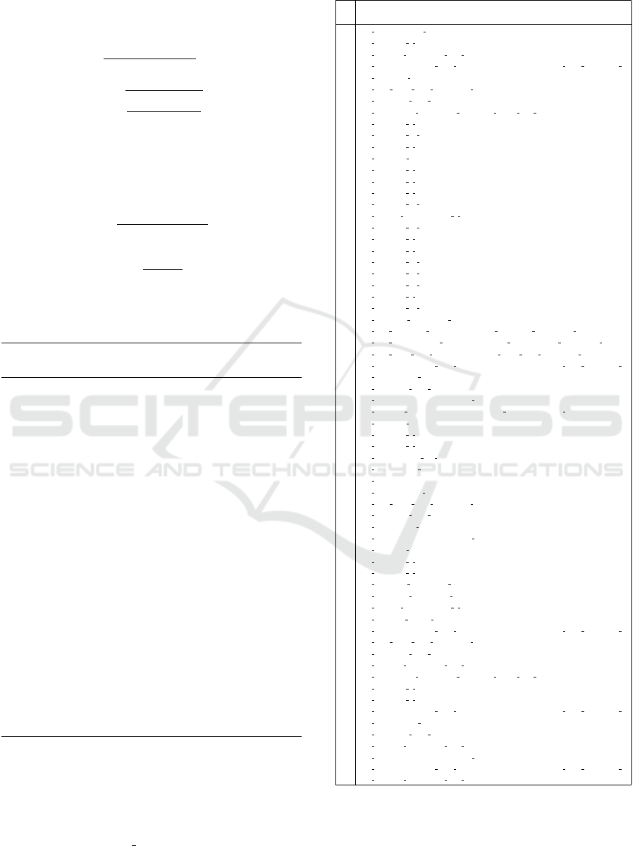
In Table 7 the subset of 66 variables after ﬁltering using

Algorithm 3 can be found. The extracted features f1, f2,

. . . , f6 refer to Eq. 14, 15, . . . , 19. The respective process

variable comes after the ” ” sign.

Table 7: Selected feature variables after ﬁltering.

no.

Features

1 f 4 schussvolumen 1

2 f 1 tempzone 3 istwert

3 f 6 drehzahl spitzenwert host 1

4 f 5 schneckenvolumen ende nachdruckcpnschneckenposition ende nachdruck 1

5 f 5 f liesszahl 1

6 f 4 hydr druck beim umschalten 1

7 f 4 entlastung ende 1

8 f 4 drehmoment spitzenwert lau f ender zyklus host 1

9 f 3 tempzone 3 istwert

10 f 1 tempzone 12 istwert

11 f 5 tempzone 5 istwert

12 f 4 zykluszeit sollwert

13 f 4 tempzone 8 istwert

14 f 4 tempzone 7 istwert

15 f 4 tempzone 6 istwert

16 f 4 tempzone 11 istwert

17 f 4 integral ueberwachung 2 micrograph

18 f 3 tempzone 11 istwert

19 f 2 tempzone 5 istwert

20 f 1 tempzone 9 istwert

21 f 1 tempzone 14 istwert

22 f 1 tempzone 13 istwert

23 f 1 tempzone 10 istwert

24 f 6 tempzone 9 istwert

25 f 6 tempzone 14 istwert

26 f 6 staudruck spitzenwert 1

27 f 6 spez nachdruck spitzenwert pnshydr nachdruck spitzenwert 1

28 f 6 spez einspritzdruck spitzenwert pvshydr eins pritzdruck s pitzenwert 1

29 f 6 spez druck beim umschaltenphuhydr druck beim umschal t en 1

30 f 6 schneckenvolumen ende nachdruckcpnschneckenposition ende nachd ruck 1

31 f 6 schliesskra f t spitzenwert

32 f 6 entlastung ende 1

33 f 6 dosiervolumenswc1dosierhub 1

34 f 6 aktuelles umschaltvolumenc3uaktuelle umschalt position 1

35 f 5 zykluszeit vollautomatik

36 f 5 tempzone 9 istwert

37 f 5 tempzone 7 istwert

38 f 5 stillstandszeit vor zyklusstart

39 f 5 schliesskra f t spitzenwert

40 f 5 ruesten

41 f 5 mengenistwert pumpe

42 f 5 hydr druck beim umschalten 1

43 f 5 entlastung ende 1

44 f 5 druckistwert pumpe

45 f 5 dosiervolumenswc1dosierhub 1

46 f 4 zykluszeit vollautomatik

47 f 4 tempzone 2 istwert

48 f 4 tempzone 1 istwert

49 f 4 staudruck spitzenwert 1

50 f 4 nachdruck spitzenwert 1

51 f 4 integral ueberwachung 1 micrograph

52 f 3 spritzzeit istwert 1

53 f 3 schneckenvolumen ende nachdruckcpnschneckenposition ende nachd ruck 1

54 f 3 hydr druck beim umschalten 1

55 f 3 entlastung ende 1

56 f 3 drehzahl spitzenwert host 1

57 f 3 drehmoment spitzenwert lau f ender zyklus host 1

58 f 2 tempzone 9 istwert

59 f 2 tempzone 7 istwert

60 f 2 schneckenvolumen ende nachdruckcpnschneckenposition ende nachd ruck 1

61 f 2 schliesskra f t spitzenwert

62 f 2 entlastung ende 1

63 f 2 drehzahl spitzenwert host 1

64 f 2 dosiervolumenswc1dosierhub 1

65 f 1 schneckenvolumen ende nachdruckcpnschneckenposition ende nachd ruck 1

66 f 1 drehzahl spitzenwert host 1

DATA 2019 - 8th International Conference on Data Science, Technology and Applications

242