Discrete-time Adaptive Regulation of Systems with Uncertain

Upper-bounded Input Delay: A State Substitution Approach

Khalid Abidi

1 a

and Hang Jian Soo

2,† b

Electrical Power Engineering Program, Newcastle University in Singapore, 567739, Singapore

National University of Singapore, 119260, Singapore

Keywords:

Adaptive Control, Discrete-time Systems, Time-delay Systems.

Abstract:

This paper proposes a discrete-time adaptive regulation approach for scalar linear time-invariant systems with

unknown, constant input time delay that has a known upper-bound, without explicitly estimating the time

delay. To cope with the unknown time delay, a state substitution is made that results in a delay free system that

simpliﬁes the control law design. In addition, the proposed approach does not require that the system have

stable open-loop zeros. A stability analysis shows that the proposed regulator drives the system state to zero

asymptotically and simulation results are shown to verify the approach.

1 INTRODUCTION

Processes with time delays at the input (i.e. delayed

control action) are encountered in many situations re-

quiring the use of feedback control, and these delays

may have signiﬁcant consequences if a controller is

not designed to compensate for them (Richard, 2003)

(Gu and Niculescu, 2003). For example, communi-

cations delays in bilateral teleoperation can cause the

force feedback loop to become unstable, possibly cre-

ating a hazard for the remote operator (Abidi et al.,

2016). In visual servoing, the computational com-

plexity of visual information processing may insert a

signiﬁcant delay into the control loop that could af-

fect stability (Bjerkeng et al., 2014). Pneumatic ac-

tuators are commonly used in soft robots, where long

pneumatic lines and the compressibility of air can in-

troduce actuator delays (Skorina et al., 2017). In all

these applications it is clear that a practical controller

must be able to cope with uncertainty in the plant pa-

rameters, including the time delay.

There are two ways to approach the problem of

compensating for input time delay. The ﬁrst ap-

proach explicitly recognises the need to predict the

future state of the system. To illustrate this, con-

sider a discrete-time time-invariant system x

k+1

f (x

k−d

) where x

is the state and u

k−d

is the time-

https://orcid.org/0000-0002-4795-5360

https://orcid.org/0000-0003-4424-4755

†

MSc student with the National University of Singapore

delayed control input. Shifting this d steps ahead, i.e.

k+d+1

= f (x

k+d

), it becomes obvious that in or-

der to affect the state at k+d +1 it would be desirable

to have knowledge of the future state at k + d. A rig-

orous argument for the case of linear time invariant

plants with a single input delay is found in (Mirkin

and Raskin, 2003). Examples of predictor-based con-

trol laws for linear and nonlinear plants are (Mani-

tius and Olbrot, 1979) (Abidi, 2014) and (Abidi and

Postlethwaite, 2019) respectively.

The second approach, commonly known as Art-

stein’s model reduction (Artstein, 1982), applies

speciﬁcally to linear, possibly time-varying systems

with input delay. A state substitution is used to trans-

form the original system into an equivalent delay-free

system, for which it is easier to derive a control law.

The control law for the former can then be found by

reversing the substitution. This in fact leads to the

same control laws as the ﬁrst approach, but it simpli-

ﬁes the derivation in the general case where there may

be multiple lumped and/or distributed input delays.

As this paper will show, it is also a useful starting

point for generalising to the case of uncertain plant

parameters and time delay.

To illustrate the method with a simple example

from (Richard, 2003), consider the linear system with

input delay ˙x(t) = Ax(t) + Bu(t − d). Introducing a

state substitution

z(t) = x(t) +

t−d

A(t−d−τ)

Bu(τ)dτ (1)

Abidi, K. and Soo, H.

Discrete-time Adaptive Regulation of Systems with Uncertain Upper-bounded Input Delay: A State Substitution Approach.

DOI: 10.5220/0007922706990706

In Proceedings of the 16th International Conference on Informatics in Control, Automation and Robotics (ICINCO 2019), pages 699-706

ISBN: 978-989-758-380-3

699

yields the equivalent delay-free system in z(t) given

˙z(t) = Az(t) + e

−Ad

Bu(t) (2)

The control law for the latter is simply a state-

feedback law u(t) = Kz(t) where K is chosen to sta-

bilise (A,e

−Ad

B). The control law for the original sys-

tem is then found by substituting the deﬁnition of z(t)

to get

u(t) = Kx(t) + K

t−d

A(t−d−τ)

Bu(τ)dτ (3)

To cope with uncertainty in the plant parameters,

including the time delay, two paradigms are available.

The ﬁrst paradigm is to make the controller robust to

the uncertainty. In delay-independent truncated pre-

dictor feedback (Wei and Lin, 2018), a state-feedback

controller is used with gains selected by a Lyapunov

equation based method which does not require knowl-

edge of the delay. However, this work assumes plant

parameters are known, and for unstable plants the

amount of delay that the method can handle is limited

(Wei and Lin, 2017). A more generally applicable but

mathematically involved alternative is to employ the

framework of robust control theory (Zhong, 2006).

The other paradigm to consider is adaptive con-

trol. Early work on adaptive controllers for time

delay systems only addressed uncertainty in the pa-

rameters but not the time delay (Ortega and Lozano,

1988)(Niculescu and Annaswamy, 2003). The reason

is that adaptive laws rely on the plant representation

being linear in the uncertain parameters, whereas the

time delay appears inside the argument of the con-

trol input. Krstic (Krstic, 2009) overcomes this by

expressing the plant dynamics in terms of the en-

tire input history over the delay interval (given by

the function u(x,t) where x parameterises a point on

the interval), and modelling the delay as a transport

PDE. Thus, the time delay can be estimated along

with other plant parameters, and used to compute a

predictor-based control law (Bresch-Pietri and Krstic,

2009). However, the resulting adaptive laws for both

time delay and parameter estimation are complicated.

Most time-delay controllers have been formulated

in a continuous-time setting, but they will almost cer-

tainly be implemented on a digital computer. Dis-

cretisation of continuous-time control laws, espe-

cially those for time-delay compensation, is fraught

with numerical pitfalls (Mirkin, 2004)(Zhong, 2004).

It may be more straightforward to design controllers

in discrete-time, for example the discrete-time APC

(Abidi et al., 2017) (Abidi and Xu, 2015). This is

a model-reference adaptive controller that achieves

reference trajectory tracking on a plant with an un-

known, constant, upper-bounded time delay. How-

ever, the model-tracking error does not vanish asymp-

totically, and its bound is dependent on the mismatch

between the delay upper-bound assumed by the con-

troller and the true delay. The adaptive law also con-

tains parameters that may be difﬁcult to tune in prac-

tice.

This paper proposes a discrete-time adaptive regu-

lator for a scalar, linear time-invariant system with an

unknown, constant input time delay that has a known

upper-bound, without explicitly estimating the time

delay. Using an approach similar to Artstein’s model

reduction, a state substitution is devised that allows

the plant dynamics to be expressed in a delay-free

form, which facilitates derivation of a control law. In

order to apply the model reduction technique to the

case of unknown time delay, the plant dynamics and

the state substitutes are expressed in a manner that is

‘agnostic’ to the speciﬁc value of the time delay. This

also makes it possible to estimate the plant parameters

using recursive least squares, even without knowledge

of the time delay. A stability analysis shows that

the proposed regulator drives the plant state to zero

asymptotically.

2 PROBLEM DEFINITION

Consider the scalar system in continuous-time with

input delay given as

˙x(t) = ax(t) + bu(t − τ) (4)

where the state is x ∈ R, the input is u ∈ R, the system

parameters a,b ∈ R are uncertain parameters, and the

constant time delay τ ∈ R is uncertain but has a known

upper-bound, τ

, such that τ ≤ τ

Sampling this system at uniform time intervals T

(where in general the time delay τ may not be an in-

teger multiple of T ) gives a discrete-time system de-

scribed by

k+1

= φx

+ γ

k−d

+ γ

k−d−1

(5)

where φ, γ

,γ

∈ R are uncertain parameters, and d ∈

[0, p] ⊂ Z

is the uncertain constant delay known

to be at most p time-steps long. It is not neces-

sary to ensure that the sampled system has stable ze-

ros, i.e., if the system is written in the form u

k−d

(−γ

k−d−1

+ x

k+1

− φx

) then the ratio

need

not be inside the unit-circle.

Assumption 1: The upper-bound on the delay in time-

steps, p, satisﬁes pT ≤ τ

≤ (p + 1)T .

Assumption 2: There exists a φ

min

> 0 such that φ ≥

min

Assumption 3: There exists a γ

min

> 0 such that γ

≥ γ

min

ICINCO 2019 - 16th International Conference on Informatics in Control, Automation and Robotics

700

The regulation problem is to ﬁnd a bounded con-

trol input u

which will drive the system state to zero

asymptotically, i.e. lim

k→∞

= 0, while keeping all

system signals bounded.

Remark 1. Since the parameter φ is computed as φ =

∀a ∈ R then it is reasonable to assume a positive

lower bound such that 0 < φ

min

≤ φ.

3 MAIN RESULT

In this section the design of the control law and adap-

tive law is presented which is then followed by a rig-

orous stability analysis of the system.

3.1 Adaptive Regulator

Consider the system (5) expressed in the form

k+1

= φx

p+1

∑

i=0

k−i

= θ

(6)

where θ



φ ψ

··· ψ

p+1



∈ R

p+3

the augmented parameter vector and ζ



··· u

k−p−1



∈ R

p+3

is the augmented

signal vector. The parameters ψ

∈ R are deﬁned as











i = d

i = d + 1

0 otherwise

i ∈ [0, p + 1] (7)

Deﬁning the variables η

and

such that

k+1

= x

k+1

p+1

∑

i=1

i,k

k−i+1

(8)

and

= x

p+1

∑

i=1

i,k

k−i

(9)

where

i,k

∈ R. Consider now the system (6), adding

and subtracting the term

on the right-hand-side,

it is obtained that

k+1

p+1

∑

i=0

k−i

(10)

where

is the estimate of φ and

, φ −

is the es-

timation error. Substitution of (9) and (10) in (8) and

adding and subtracting the term

0,k

on the right-

hand-side results in the delay free dynamics of the

form

k+1

0,k

−

0,k

−

p+1

∑

i=0

i,k

k−i

p+1

∑

i=0

k−i

p+1

∑

i=1

i,k

k−i+1

p+1

∑

i=0

k−i

−



0,k

−

1,k



−

∑

i=1



i,k

−

i+1,k



k−i

−

p+1,k

k−p−1

0,k

p+1

∑

i=0

k−i

−

p+1

∑

i=0

i,k

k−i

0,k

(11)

where the adaptive parameters

i,k

are the estimates

of ψ

and are deﬁned as

i,k











0,k

−

1,k

i = 0

i,k

−

i+1,k

i ∈ [1, p]

i,k

i = p + 1

(12)

Note that the parameters

i,k

∀i ∈ [0, p + 1] are com-

puted from the adaptative parameters as

i,k











p+1

∑

j=0

− j

j,k

i = 0

p+1

∑

j=i

− j+i−1

j,k

i ∈ [1, p + 1]

(13)

which is obtained by rearranging (12). Finally, deﬁn-

ing

i,k

, ψ

−

i,k

such that (11) is written as

k+1

p+1

∑

i=0

i,k

k−i

0,k

(14)

where

, θ −

is the augmented parameter esti-

mation error vector and



0,k

···

p+1,k



∈

p+3

is the augmented adaptive parameter vector,

then from (14), the control law is selected as

= −

−1

0,k

(15)

With the formulation of the control law completed,

the adaptive law can be derived.

Remark 2. Note that the inverses of

0,k

and

are

needed in (15) and (13), therefore, the adaptive law

must ensure that those terms are non-singular.

Proceeding with the adaptive law derivation, con-

sider the system (14) and the control law (15). Sub-

stitution of the control law results in the closed-loop

dynamics

k+1

(16)

Discrete-time Adaptive Regulation of Systems with Uncertain Upper-bounded Input Delay: A State Substitution Approach

701

From (16), the adaptive law is selected as









k−1

+ P

k−1



∀k ∈ (k

,∞)

∀k ∈ [0, k

]

(17)











k−1

−

k−1

1 + ζ

k−1

∀k ∈ (k

,∞)

∀k ∈ [0, k

]

(18)

where k

≥ 0 is the initial time-step, P

∈ R

p+3×p+3

is the symmetric positive-deﬁnite covariance matrix.

The purpose of the operator L[·] is to keep

and

0,k

non-singular. The deﬁnition of the operator L [·] for

is given as

L [

] =

(

∈ (φ

min

,∞)

min

∈ (−∞, φ

min

]

(19)

Before proceeding with the deﬁnition of the operator

L [·] for



0,k

···

p+1,k



, consider (13) and note that

for i = 0

0,k

p+1

∑

j=0

− j

j,k

. (20)

Since

> φ

min

and ideally

j,k

≥ 0, then the only

possibility for a singular

0,k

is if the adaptive param-

eters

j,k

= 0, ∀ j ∈ [0, p + 1]. Therefore, the operator

L [·] will need to be deﬁned under two scenarios. In

the ﬁrst scenario, consider the case that one or more

but not all adaptive parameters

j,k

are smaller than

or equal to zero, which leads to the L[·] being deﬁned



j,k



(

j,k

∈ (0, ∞)

j,k

∈ (−∞, 0]

(21)

for all j ∈ [0, p + 1]. In the second scenario, con-

sider the case when all the adaptive parameters

j,k

are smaller than or equal to zero, then the operator

L [·] is deﬁned as



j,k



min

p + 2

(22)

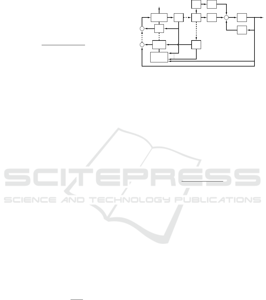
for all j ∈ [0, p + 1]. The block diagram of the result-

ing closed-loop system is shown in Fig. 1. Note that

in Fig. 1 the delay-operator is represented by q

−1

Remark 3. Note that since the delay d is uncertain,

it is not possible to assign the lower bound on γ

,γ

correctly in the case when all the values

j,k

≤ 0.

Therefore, the average value of the lower bound γ

min

is assigned to every

j,k

−β

−1

0,k

−1

1,k

p+1,k

−1

Adaptive

Law

d + 1

delay

p + 1

delay

ˆη

k+1

Figure 1: Block diagram depicting the proposed adaptive

regulator connected to the system.

3.2 Stability Analysis

In this section, it is shown that the parameter adapta-

tion produces bounded and convergent parameter es-

timates (Lemma 1), that the adaptive system model

converges in input-output behaviour to the true sys-

tem (Lemma 2), and that the proposed adaptive reg-

ulator drives the system state to zero with vanishing

control effort (Theorem 3).

Lemma 1. For the system (16) with the adaptive laws

(17) and (18) it is true that

lim

k→∞

1 + ζ

k−1

= 0 (23)

Furthermore, it is also true that the parameter estimate

is bounded, hence the parameter estimation error

is also bounded.

Proof. Consider the positive function

−1

(24)

The backward difference ∆V

∆V

= V

−V

k−1

−1

−

k−1

−1

k−1

(25)

Using the fact that, (Abidi and Xu, 2008),



θ − L







θ − L





≤



θ −





θ −



(26)

and that if P

−1

is positive-deﬁnite then it is obtained

that



θ − L





−1



θ − L





≤



θ −



−1



θ −



(27)

Substituting the (27) and the adaptative law (17) in

ICINCO 2019 - 16th International Conference on Informatics in Control, Automation and Robotics

702

(25) leads to

∆V

= V

−V

k−1



k−1

− P

k−1



−1



k−1

− P

k−1



−

k−1

−1

k−1

−1

k−1

−

k−1

−1

k−1

−

k−1

−1

× (P

k−1

) − (P

k−1

)

−1

k−1

+ (P

k−1

)

−1

k−1

)

k−1

−1

− P

−1

k−1

)

k−1

− 2

k−1

+ ζ

k−1

(28)

and using the fact that P

−1

= P

−1

k−1

+ζ

k−1

, (Abidi

et al., 2017), it is obtained that (28) is simpliﬁed to

the form

∆V

k−1

− 2

k−1

+ ζ

k−1

(29)

Substituting in the model estimation error dynamics

(16) gives

∆V

= η

− 2η

+ ζ

k−1

= η

[−1 + ζ

k−1

] (30)

Furthermore, from (18) it is obtained that

k−1

1 + ζ

k−1

(31)

Substitution of (31) in (30) ﬁnally leads to

∆V

= η

−1 +

k−1

1 + ζ

k−1

= −

1 + ζ

k−1

(32)

From the result (32) it is evident that ∆V

is always

non-positive and, hence V

, is non-increasing. There-

fore, the parameter estimation error

and the param-

eter estimate

are bounded. Furthermore, the value

of V

is the accumulation of changes ∆V

to its initial

value V

= V

k−k

∑

i=1

∆V

(33)

Substituting (32) into (33) gives

= V

−

k−k

∑

i=1

1 + ζ

i−1

(34)

and using the result in (Abidi et al., 2017) it is con-

cluded that

lim

k→∞

∆V

= lim

k→∞

1 + ζ

k−1

= 0 (35)

Lemma 2. From Lemma 1, for the signals (8) and (9)

the following are true:

(a) |x

| ≤ c

max

i∈[0,p+1]

k−i

|, for some positive

constant c

(b) |

| ≤ d

+ d

max

i∈[0,p+1]

|η

k−i

|, for some posi-

tive constants d

and d

k→∞

= η

(d) lim

k→∞

= 0 and lim

k→∞

= 0.

Proof. Consider the signal (9) re-written as

−

p+1

∑

i=1

i,k

k−i

(36)

Substitution of the control law (15), it is obtained as

p+1

∑

i=1

i,k

−1

0,k−i

k−i

(37)

In Lemma 1 it is established that the adaptive param-

eters are bounded which implies that

i,k

−1

0,k−i

k−i

is bounded. Using the boundedness of the adaptive

paramters in (37), it is obtained that

| ≤ |

| +

p+1

∑

i=1

i,k

−1

0,k−i

k−i

≤ c

max

i∈[0,p+1]

k−i

| (38)

for some positive constant c

Consider now the difference of the two signals (9)

and (8) given as

= −

p+1

∑

i=1



i,k

−

i,k−1



k−i

+ η

p+1

∑

i=1



i,k

−

i,k−1



−1

0,k−i

k−i

+ η

(39)

Expressing this in augmented form and deﬁning

i,k

−1

0,k−i

k−i

(

i,k

−

i,k−1

) such that,







1,k

2,k

···

p+1,k

1 0 ··· 0

0 1 ···







k−1













(40)

where

k−1



k−1

···

k−p



. From Lemma

1 and using the results in (Abidi et al., 2017),

lim

k→∞

−1

0,k−i

k−i

(

i,k

−

i,k−1

) = 0 and that implies

that the augmented system (40) is stable and a bound

exists such that

| ≤ d

+ d

max

i∈[0,p+1]

|η

k−i

| (41)

Discrete-time Adaptive Regulation of Systems with Uncertain Upper-bounded Input Delay: A State Substitution Approach

703

for some positive constants d

and d

Going back to the augmented system (40), at

steady state when k → ∞, the term

−1

0,k−i

k−i

(

i,k

−

i,k−1

) will vanish resulting in an augmented system

of the form







0 0 ··· 0

1 0 ··· 0

0 1 ···







k−1













(42)

which has a solution

= η

when k → ∞.

Finally, given the result in (35), the Key Tech-

nical Lemma states that η

vanishes if there exists

positive constants µ

,µ

∈ R such that |ζ

k−1

| ≤ µ

max

κ∈[0,k]

|η

|. To show that this is indeed true,

recall that ζ



··· u

k−p−1



. It has been es-

tablished that |x

| ≤ c

max

i∈[0,p+1]

k−i

| and, since,

−1

0,k−i

k−i

is bounded then |u

| ≤ c

|. There-

fore, |ζ

k−1

| ≤ µ

+µ

max

κ∈[0,k]

|η

| for some positive

constants µ

and µ

and, ultimately, lim

k→∞

= 0.

Furthermore, from (c) it has been established that

lim

k→∞

= η

resulting in lim

k→∞

= 0.

Theorem 1. The state of the closed-loop system, as

well as the control signal, approach zero asymptoti-

cally, i.e. lim

k→∞

= lim

k→∞

= 0.

Proof. Beginning with the closed-loop controller dy-

namics (15) and taking the limit of the norm of both

sides as k → ∞, it is obtained that

lim

k→∞

= lim

k→∞



−

−1

0,k



≤ lim

k→∞



−1

0,k



= 0 (43)

Consider now the expression (8) as k → ∞ which is

given as

lim

k→∞

| ≤ lim

k→∞

| + lim

k→∞

p+1

∑

i=1

i,k

k−i

= 0 (44)

which establishes the asymptotic stability of the state

4 SIMULATION EXAMPLE

Consider an unstable system with an unstable zero,

given by

k+1

= 1.05x

+ 1u

k−d

+ 1.1u

k−d−1

(45)

where the system delay is set as d = 0, 1, 2, 3, 4, 5

while the upper bound is set as p = 5. The initial

condition of the system is set at x

= 2.

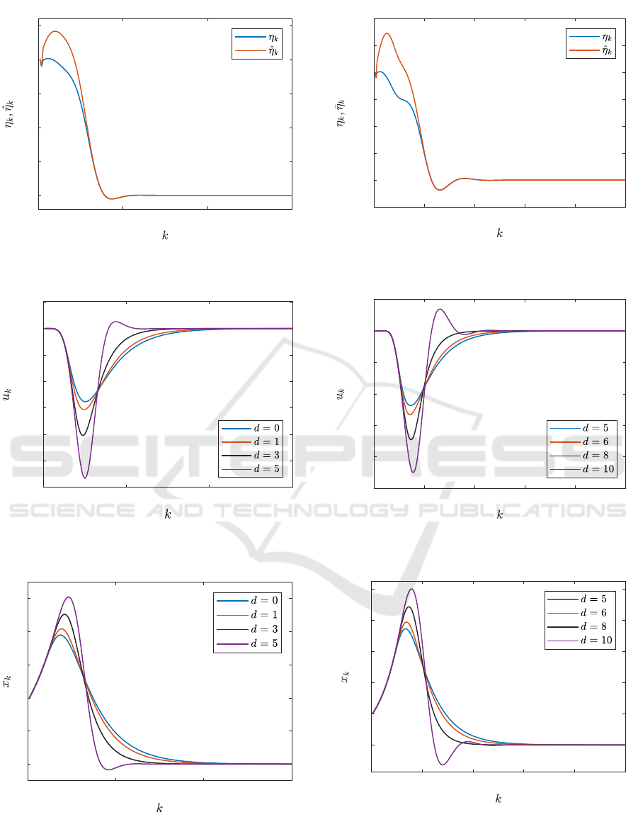
To investigate the adaptive performance of the

regulator with respect to mismatch between the de-

lay upper-bound p and the true delay d, the closed-

loop system is simulated using various values of d.

The adaptive regulator is initialised with P

= 5 ×

p+3×p+3

and



0.1 0.4 ··· 0.4



. In Fig. 2-4 the

results are shown for the convergence of the signals

, the control input proﬁle and state regulation

performance of the closed-loop system under various

values of the delay values. As expected, x

is regu-

lated to zero asymptotically. As it can be seen from

the results, the greater the mismatch between p and d,

the longer the settling-time. Note that with increasing

system delay, d, the initial divergence grows which

is to be expected as the controller cannot react fast

enough initially to force the system to converge.

Finally, the system is simulated with a longer sys-

tem delay, d, and an upper bound set at p = 10. The

adaptive regulator parameters are kept the same as

the previous case while the system delay is increased

from d = 5 until d = 10. The results are shown in

Fig. 5-7. The results for this case show a similar per-

formance to the shorter delay case. As it would be

expected, the convergence speed increases as the ac-

tual delay, d, and the upper bound, p, approach each

other.

5 CONCLUSIONS

In this paper, a discrete-time adaptive regulation ap-

proach was designed for a scalar system with an

unknown, constant time-delay with a known upper-

bound. The approach utilized a state substitution the

resulted in a delay-free system which simpliﬁed the

control law design. The approach is also capable of

handling systems with unstable zeros. A rigorous

stability proof was presented that shows the adaptive

control law drives the system state to zero asymptoti-

cally. Finally, numerical simulations were shown that

illustrate the ability of the adaptive control law to cope

with mismatches between the delay upper-bound and

the true delay in the system.

ICINCO 2019 - 16th International Conference on Informatics in Control, Automation and Robotics

704

0 50 100 150

0.5

1.5

2.5

Figure 2: Asymptotic convergence of η

and

when d = 5

and p = 5.

0 50 100 150

-0.3

-0.25

-0.2

-0.15

-0.1

-0.05

0.05

Figure 3: Control input proﬁle on the system when p = 5,

with various values of the actual system delay d.

0 50 100 150

Figure 4: State regulation of the system when p = 5, with

various values of the actual system delay d.

0 50 100 150 200 250

-0.5

0.5

1.5

2.5

Figure 5: Asymptotic convergence of η

and

when d =

10 and p = 10.

0 50 100 150 200 250

-0.5

-0.4

-0.3

-0.2

-0.1

0.1

Figure 6: Control input proﬁle on the system when p = 10,

with various values of the actual system delay d.

0 50 100 150 200 250

Figure 7: State regulation of the system when p = 10, with

various values of the actual system delay d.

Discrete-time Adaptive Regulation of Systems with Uncertain Upper-bounded Input Delay: A State Substitution Approach

705

REFERENCES

Abidi, K. (2014). A robust discrete-time adaptive con-

trol approach for systems with almost periodic time-

varying parameters. International Journal of Robust

and Nonlinear Control, 24(1):166–178.

Abidi, K. and Postlethwaite, I. (2019). Discrete-time adap-

tive control for systems with input time-delay and

non-sector bounded nonlinear functions. IEEE Ac-

cess, 7:4327–4337.

Abidi, K. and Xu, J. (2008). A discrete-time periodic

adaptive control approach for time-varying parame-

ters with known periodicity. IEEE Transactions on

Automatic Control, 53(2):575–581.

Abidi, K. and Xu, J. X. (2015). Advanced Discrete-Time

Control: Designs and Applications. Springer.

Abidi, K., Yildiz, Y., and Annaswamy, A. (2017). Con-

trol of uncertain sampled-data systems: An adaptive

posicast control approach. IEEE Transactions on Au-

tomatic Control, 62(5):2597–2602.

Abidi, K., Yildiz, Y., and Korpe, B. E. (2016). Explicit

time-delay compensation in teleoperation: An adap-

tive control approach. International Journal of Robust

and Nonlinear Control, 26(15):3388–3403.

Artstein, Z. (1982). Linear systems with delayed controls:

A reduction. IEEE Transactions on Automatic Con-

trol, 27(4):869–879.

Bjerkeng, M., Falco, P., Natale, C., and Pettersen, K. Y.

(2014). Stability analysis of a hierarchical architec-

ture for discrete-time sensor-based control of robotic

systems. IEEE Transactions on Robotics, 30(3):745–

753.

Bresch-Pietri, D. and Krstic, M. (2009). Adaptive trajec-

tory tracking despite unknown input delay and plant

parameters. Automatica, 45(9):2074–2081.

Gu, K. and Niculescu, S. (2003). Survey on recent results in

the stability and control of time-delay systems. Jour-

nal of Dynamic Systems, Measurement, and Control,

125(2):158–165.

Krstic, M. (2009). Delay Compensation for Nonlinear,

Adaptive, and PDE Systems. Birkh

auser.

Manitius, A. and Olbrot, A. (1979). Finite spectrum assign-

ment problem for systems with delays. IEEE Trans-

actions on Automatic Control, 24(4):541–552.

Mirkin, L. (2004). On the approximation of distributed-

delay control laws. Systems & Control Letters,

51(5):331–342.

Mirkin, L. and Raskin, N. (2003). Every stabilizing dead-

time controller has an observer-predictor-based struc-

ture. Automatica, 39(10):1747–1754.

Niculescu, S. and Annaswamy, A. M. (2003). An adaptive

smith-controller for time-delay systems with relative

degree n

∗

≤ 2. Systems & Control Letters, 49(5):347–

358.

Ortega, R. and Lozano, R. (1988). Globally stable adap-

tive controller for systems with delay. International

Journal of Control, 47(1):17–23.

Richard, J. (2003). Time-delay systems: An overview of

some recent advances and open problems. Automat-

ica, 39(10):1667–1694.

Skorina, E. H., Luo, M., Tao, W., Chen, F., Fu, J., and Onal,

C. D. (2017). Adapting to ﬂexibility: Model refer-

ence adaptive control of soft bending actuators. IEEE

Robotics and Automation Letters, 2(2):964–970.

Wei, Y. and Lin, Z. (2017). Maximum delay bounds of lin-

ear systems under delay independent truncated predic-

tor feedback. Automatica, 83:65–72.

Wei, Y. and Lin, Z. (2018). Stability criteria of linear sys-

tems with multiple input delays under truncated pre-

dictor feedback. Systems & Control Letters, 111:9–17.

Zhong, Q. (2004). On distributed delay in linear control

laws – part i: discrete-delay implementations. IEEE

Transactions on Automatic Control, 49(11):2074–

2080.

Zhong, Q. (2006). Robust Control of Time-Delay Systems.

Springer.

ICINCO 2019 - 16th International Conference on Informatics in Control, Automation and Robotics

706