Computational Fluid Dynamics Model for Sensitivity Analysis and

Design of Flow Conditioners

V. Askari, D. Nicolas, M. Edralin and C. Jang

British Columbia Institute of Technology, School of Energy, Department of Mechanical Engineering,

3700 Willingdon Avenue, Burnaby, BC, Canada

Keywords: Computational Fluid Dynamics, Flow Conditioner, Swirling Flow, Flow Measurement, Flow Velocity Profile.

Abstract: Flow conditioners are used to measure flow rate more accurately. The sensitivity of flow measurement devices

to swirling flows and not fully developed flows are subjects of concerns to flowmeter manufacturers as well

as industries. Inaccurate flow measurement occurs in the presence of swirl flow and when the flow velocity

profile is not fully developed. Distorted profiles occur when the piping configuration upstream of the flow

measurement devices changes. Certain length of straight piping upstream of a flow meter is required to

achieve acceptable flow velocity profile for expected flow meter accuracy. In some installations, it is not

realistic to run lengths of piping to reach an acceptable flow velocity profile. Introducing flow conditioners

into the system reduces piping needed to reach fully developed flow and significantly weaken swirling flows.

In this study, a Computational Fluid Dynamics (CFD) model is developed and validated which is used to

investigate systematically the sensitivity of various parameters for perforated flow conditioners. Published

data and an experimental setup was used to verify the CFD model.

1 INTRODUCTION

Flow conditioners are used for homogenizing the

velocity profile, as well as removing swirls, created

by disturbances. Installations such as elbows and

double elbows, create swirls in the flow that can result

in inaccurate measurements by the flow meters. It is

essential the use of a flow conditioner to remove

disturbances in the flow, enabling proper

performance of the flow meter. Most flowmeters are

calibrated under conditions of fully developed flow.

Typically, without a flow conditioner it can take

approximately 30 L/D to obtain acceptable flow

profile for the measurement devices. Adding long

straight piping can be costly, and use up large

amounts of space. Using a flow conditioner

accelerates the development of flow profile as well

while also fading swirls. There are certain standards,

specifically ISO 5167, which define acceptable fully

developed flow, free from swirls and pulsations. The

standard states that, swirl-free conditions are

presumed “to exist when the swirl angle at all points

over the pipe cross-section is less than 2° (ISO,

2003).” The acceptable flow conditions exist when,

“at each point across the pipe cross-section, the ratio

of the local axial velocity to the maximum axial

velocity at the cross-section agrees to within ±5%

which would be achieved in swirl-free flow at the

same radial position at a cross-section located at the

end of a very long straight length L/D>100 of similar

pipe (ISO, 2003).”

The purpose of this project was to investigate the

performance of current perforated flow conditioners,

and to design and build a CFD model as a test bench

using academic COMSOL® Multiphysics software.

The CFD model is used to further investigate the

performance of the perforated flow conditioners and

sensitivity of the design parameters.

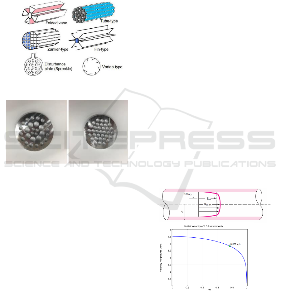
2 FLOW CONDITIONERS

There are various types of flow conditioners such as

those shown in Figure 1. However, for this study, two

perforated flow conditioners shown in Figure 2 are

examined. The perforated flow conditioner is chosen

over the other types due to its most used in industry

and ease of installation. Flow conditioners that

require long lengths of piping such as the tube-type

flow conditioner is effective in removing

disturbances in flow, but it is not ideal for

applications that are limited by space. In addition,

Askari, V., Nicolas, D., Edralin, M. and Jang, C.

Computational Fluid Dynamics Model for Sensitivity Analysis and Design of Flow Conditioners.

DOI: 10.5220/0007917401290140

In Proceedings of the 9th International Conference on Simulation and Modeling Methodologies, Technologies and Applications (SIMULTECH 2019), pages 129-140

ISBN: 978-989-758-381-0

129

maintenance is not as user-friendly for these types of

flow conditioners. In order to compare CFD results

with published data, the data from the study of

comparison of velocity and turbulence profiles

downstream of NEL and Mitsubishi perforated plate

conditioner were used for CFD model verification

and validation (Spearman, 1996).

Figure 1: Different types of flow conditioners (Miller,

1996).

Figure 2: Perforated flow conditioners. Left: NEL

Spearman, Right: Mitsubishi.

3 COMPUTATIONAL FLUID

DYNAMICS MODEL

A CFD model was developed and compared with

published experimental data. The same parameters

used in previous works (Spearman, 1996) such as

flow rate of 40 L/s and internal pipe diameter of 102.6

mm were used for the CFD model to study two types

of upstream disturbances: i) a single 90 elbow, and

ii) a double out of plane 90  elbows. Both

disturbances had a bend radius to diameter ratio (R/D)

of 1.5. Flow conditioners were placed 4 L/D

downstream of flow disturbing installations.

Measurements of velocity profiles were made at 3, 6,

11, 16, 21, 26, 31, 36 and 41 L/D downstream of each

flow conditioner. These points correspond to 7, 10,

15, 20, 25, 30, 35, 40 and 45 L/D downstream of the

disturbance. In addition, we used the Reynolds

Averaged Navier-Stokes (RANS) turbulence using

the standard k- model available in the COMSOL

software. There are other RANS models such as k-

model; there are of advantages and disadvantages

when comparing two models (Drainy, 2009). The k-

model was used because of software and hardware

limitations (Argyropoulos, 2015).

3.1 CFD Approach

Modelling the full configuration in 3D would require

a lot of computing power, and will take extremely

long time to run the simulation. Moreover, due to the

limitations on academic version of COMSOL

software, the model was broken up into two parts: a

2D axisymmetric model simulating the 77 L/D pipe

upstream of the disturbance, and 3D model

simulating the disturbance and the 48 L/D test

section. The flat velocity profile as an inlet condition

for 2D model eventually becomes fully developed at

the end of the 2D model section. The outlet velocity

profile of 2D model is then used as the inlet velocity

for the 3D model. Turbulent kinetic energy, and

turbulent dissipation rate is also derived from the

straight section, which is used as part of the inlet

condition.

The first step in verifying the results from CFD was

to check the velocity profile at the end of the straight

section of 2D model. If the velocity profile is fully

developed, the velocity at the point 0.216



from the

wall (where 



is the radius of the pipe), should be

equal to the average velocity which in this case, the

average velocity should equal the inlet velocity of

4.8381 m/s (Figure 3).

Figure 3: Velocity profile at outlet of 2D model

avg

=4.8375 m/s).

The second step in verification is to compare the

velocity profiles of the CFD model with both the

Mitsubishi and NEL Spearman flow conditioner

SIMULTECH 2019 - 9th International Conference on Simulation and Modeling Methodologies, Technologies and Applications

130

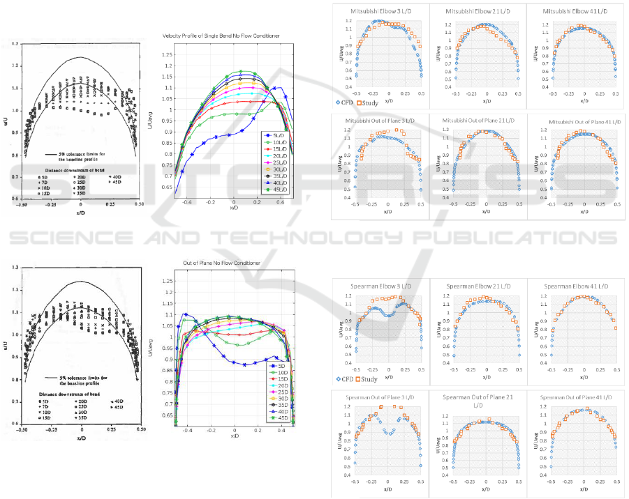
published data. The comparisons were made between

the overall shape of the velocity profile, as well as

percent error between similar points. Typically, the

velocity profile data is plotted non-dimensionally

with respect to the mean pipe velocity 



, to allow

for comparison regardless of configuration inputs. An

average percent error was taken between the points.

These points were taken at five locations, at the

centre, ±0.3 x/D, and ±0.4 x/D. Figure 4 and Figure 5

give a general comparison of the overall velocity

profile shape, for both configurations without any

flow conditioner. The overall shape from the CFD

results follow the published data, with differences in

magnitude closer to the wall. At the end of the pipe,

the velocity profile closely matches each other. The

peak is roughly 1.16 from the CFD model, versus

1.15 from the study.

Figure 4: Velocity profile (single 90 elbow).

Figure 5: Velocity profile (double out of plane 90 elbows).

Figure 6 and Figure 7 show the individual comparison

between the velocity profile from the CFD model and

the study downstream of flow conditioners. The

expectation was that, at the end of the test section the

velocity profiles should be fairly similar to that of the

study. Moving upstream from the end of the pipe, the

accuracy and similarities should slightly decrease.

From Figure 6, the Mitsubishi flow conditioner was

expected to have some asymmetry. There is some

asymmetry from the CFD, but eventually becomes

symmetric further downstream. The asymmetry is

more prominent at lower L/D values, such as 11 L/D

(see Appendix). The average error obtained from the

single elbow Mitsubishi velocity profile plots was

±3.81%. Judging by the overall shape of the velocity

profile, as well as the average error obtained, there is

strong evidence that the CFD model can correctly

predict the flow patterns. Similar to the elbow, the

double elbow configuration flowing through the

Mitsubishi should show some asymmetry. The error

for this configuration running through the Mitsubishi

flow conditioner was ±4.12%.

Figure 6: Velocity profile Mitsubishi: top: single 90 

elbow, bottom: double out of plane 90 elbows.

Figure 7: Velocity profile NEL Spearman: top: single 90

elbow, bottom: double out of plane 90 elbows.

Computational Fluid Dynamics Model for Sensitivity Analysis and Design of Flow Conditioners

131

4 PERFORMANCE ANALYSIS

The velocity profile and the swirl results for both

Mitsubishi and Spearman flow conditioners CFD

modelling using COMSOL

are presented in this

section.

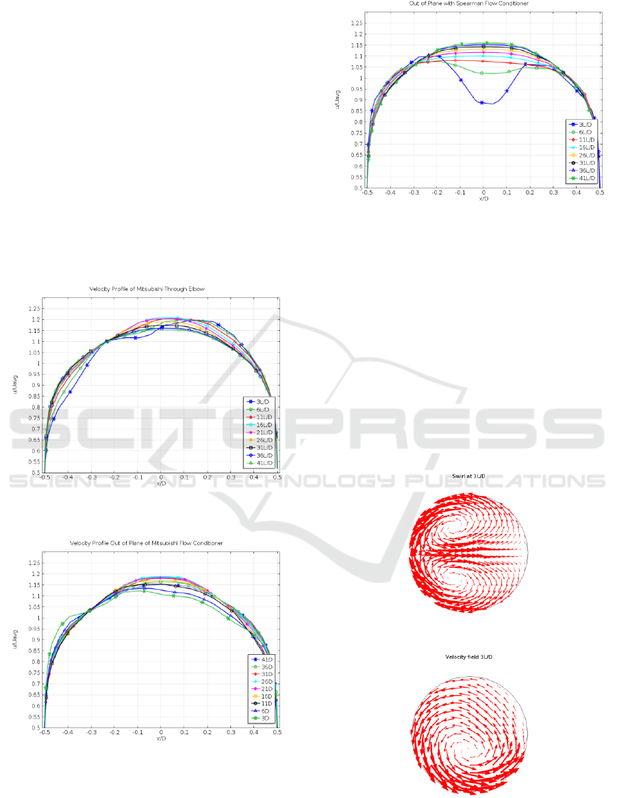
4.1 Velocity Profile

The Mitsubishi flow conditioner shows some

asymmetry from 3 to 21 L/D (Figure 8 and Figure 9).

Further, downstream the velocity profiles seems to

become more symmetrical. While it may look as if the

velocity profiles are within the acceptable tolerance of

ISO 5167 (ISO, 2003), the study reports that even at 41

L/D the velocity profile does not meet the

requirements.

Figure 8: Velocity profiles downstream of Mitsubishi flow

conditioner (single 90 elbow).

Figure 9: Velocity profiles downstream of Mitsubishi flow

conditioner (double out of plane 90 elbows).

Figure 10 shows the profiles from the NEL Spearman

flow conditioner through a double elbow. The results

show that the performance of the NEL Spearman flow

conditioner is comparable to that of the Mitsubishi.

Figure 10: Velocity profiles downstream of NEL Spearman

flow conditioner (double out of plane 90 elbows).

4.2 Swirls

For the accurate flow measurement, stable flow is

required. The flow in any piping system is sensitive to

upstream piping/fittings and devices that cause

distortion not only on flow profile, but also may

produce swirling flow that affects the accuracy of any

flow measurement devices. By installing flow

conditioners, the earlier mixing would take place

resulting of fading the swirl and achieving the fully

developed velocity profile in shorter L/D distance.

Figure 11 and Figure 12 show the velocity filed (swirl)

for a single and double out of plane 90 elbows.

Figure 11: Velocity field through 90 elbow (Re=1.5E6).

Figure 12: Velocity field through double out of plane 90

elbows (Re=1.5E6).

SIMULTECH 2019 - 9th International Conference on Simulation and Modeling Methodologies, Technologies and Applications

132

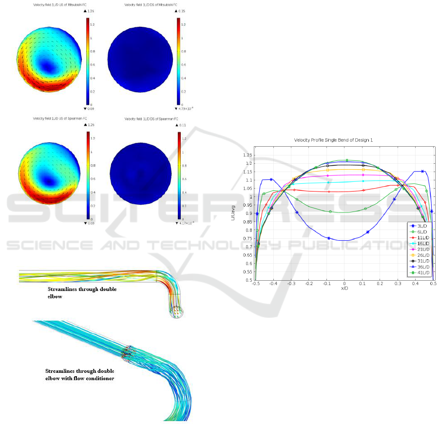
To compare the effectiveness in the removal of swirls,

the analysis will include only the double elbow

configuration. The comparison will be analysed at 1

L/D upstream, and 1 L/D downstream of the flow

conditioner. Figure 13 shows that both flow

conditioners are effective in removing swirls from the

system. Upstream of the flow conditioner, the

maximum velocity of the swirl was 1.26 m/s. After

Figure 13: Velocity field upstream (US) and downstream

(DS) of flow conditioners.

Figure 14: Velocity field US and DS of flow conditioners.

just 1 L/D downstream, the magnitude of the swirl

significantly decreases, to a maximum velocity of

0.11 m/s. It is clear that, regardless of flow

conditioner, the swirls are removed. The swirls can

also be seen through streamlines in Figure 14, which

die out relatively slowly. In contrast, the flow

conditioner removes the swirls.

4.3 Flow Conditioner Modification and

Results

Using the CFD model, a sensitivity analysis was

performed on modified flow conditioner. The

approach used in modifying the flow conditioner was

to first select one flow conditioner, and change

parameters such as the position of the holes, size,

shape, and percentage porosity. The chosen flow

conditioner to modify was the NEL Spearman,

because there was room for improvement in terms of

the geometry.

The corresponding velocity profiles for different

modified NEL Spearman flow conditioner are shown

in Figure 15-Figure 18. Design 1 configuration (Figure

15) produces a larger trough near the middle of the

pipe.

Figure 15: Design 1 velocity profile.

Due to the decreased hole size near the middle in

design 1, more fluid flows through the outer portion,

which is conveyed by the two crests near the wall. By

decreasing the porosity, the pressure drop increased,

which was expected. Moving away from the initial

method of increasing the outer holes, while

decreasing the inner ones, the next modification

(design 2-4) was attempted to allow for more flow in

the middle, rather than the outer. By this design

change, the more turbulent flow is forced to mix with

the less turbulent flow. As a result, the corresponding

highest porosity is 56.7% for design 3, which is closer

to the Mitsubishi porosity value. The dimensions and

location of the holes for all four designs are presented

in Appendix.

This iteration (design 3) has shown better

performance than the first design, but both designs

Computational Fluid Dynamics Model for Sensitivity Analysis and Design of Flow Conditioners

133

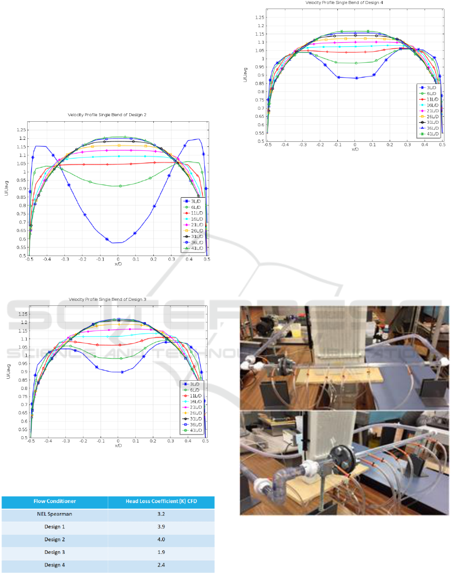
obtain fully developed flow at 21 L/D, which is

higher than the benchmarked flow conditioners.

However, this design has proved that increasing the

flow through the centre, is more beneficial. There is

slight asymmetry shown on the velocity profiles

(Figure 17), which disappears after 21L/D. Table 1

shows the head loss coefficient for all four designs.

The head loss coefficient for design 3 was lowest

value, at a value of 1.9.

Figure 16: Design 2 velocity profile.

Figure 17: Design 3 velocity profile.

Table 1: Head loss coefficient comparison.

Figure 18: Design 4 velocity profile.

4.4 Experimental Setup

A mini pilot-scale model flow loop is used to test the

flow conditioners. The experimental setup is one of

the most important aspects of any computational fluid

modelling verification and validation. A centrifugal

pump and a turbine flow meter used to build the

model. The same piping configurations as

computational model with disturbances and flow

conditioners used for experimental setup.

Figure 19: top: Flow loop with a single 90 elbow and

bottom: double out of plane 90 elbows.

Figure 19 shows the two tested piping configurations

with a flange for inserting the flow conditioner

downstream of the disturbance. In addition, to find

the effects of a flow conditioner, nine pressure taps

were added on the piping (Figure 19) with the tap

locations listed in Table 2.

SIMULTECH 2019 - 9th International Conference on Simulation and Modeling Methodologies, Technologies and Applications

134

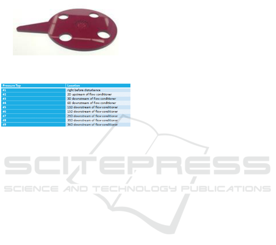
For this experimental setup, the flow conditioners

manufactured using the laser-cutting machine (Figure

20).

Figure 20: Manufactured flow conditioner.

Table 2: Location of pressure taps.

Along with verification through recreating past-

published studies, COMSOL

models also were

verified by comparing the differential pressures found

through the experimental flow loop. The results show

the same trend but a modified experimental setup is

required to achieve a higher accuracy in comparison

the results, which is a part of future activities.

5 CONCLUSION

COMSOL software is used to build a CFD model to

investigate the performance of perforated flow

conditioners with different designs. The model was

verified and validated using published data for NEL

Spearman and Mitsubishi flow conditioners. Using

the developed model, the sensitivity on the

performance of modifying parameters such as,

thickness, size, position, and shape of the holes, were

examined to develop a new perforated flow

conditioner and to compare with NEL Spearman and

Mitsubishi flow conditioners. The experimental flow

loop was used to verify the COMSOL

models. The

loop was designed to support testing for two upstream

disturbances; i) an in-plane elbow disturbance, and ii)

an out of plane elbow disturbance. Both setups

emulate the two COMSOL

models. Needed

improvements to the experimental flow loop will help

in providing more accurate results and decreasing

discrepancies due to physical limitations. The

combination of computational model verified by

experimental data can be considered as an efficient

way for sensitivity analysis of flow conditioners and

designing new flow conditioners.

REFERENCES

Argyropoulos, C.D., Markatos, N.C., 2015. Recent

advances on the numerical modelling of turbulent

flows. Applied Mathematical Modelling Journal,

Elsevier.

Drainy, Y. A., 2009. CFD Analysis of Incompressible

Turbulent Swirling Flow through Zanker Plate. Journal

of Engineering Applications of Computational Fluid

Mechanics.

ISO, 2003. Measurement of Fluid Flow by Means of

Pressure Differential Devices inserted in Circular

Cross-section Conduits Running Full. International

Organization for Standardization

Miller, R. W., 1996. Flow Measurement Engineering

Handbook, 3

edition: McGraw-Hill.

Spearman, M., 1996. Comparison of velocity and

turbulence profiles downstream of perforated plate

flow conditioners. Flow Measurement and

Instrumentation, Vol. 7.

Computational Fluid Dynamics Model for Sensitivity Analysis and Design of Flow Conditioners

135

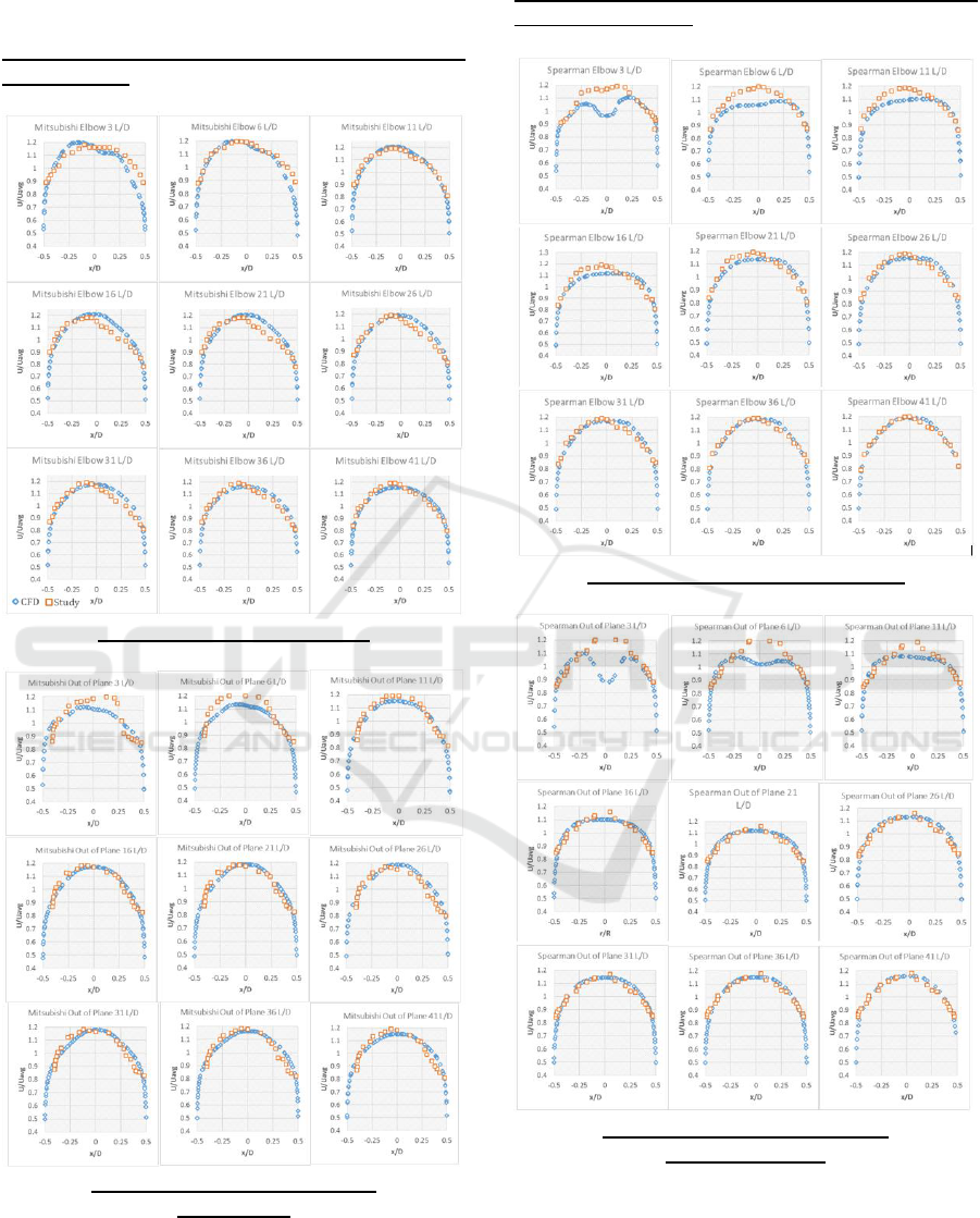
APPENDIX

Velocity Profile Comparison (Mitsubishi Flow

Conditioner):

Single 90 elbow (Mitsubishi)

Double out of plane 90 elbows

(Mitsubishi)

Velocity Profile Comparison (NEL Spearman

Flow Conditioner):

Single 90 elbow (NEL Spearman)

Double out of plane 90 elbows

(NEL Spearman)

SIMULTECH 2019 - 9th International Conference on Simulation and Modeling Methodologies, Technologies and Applications

136

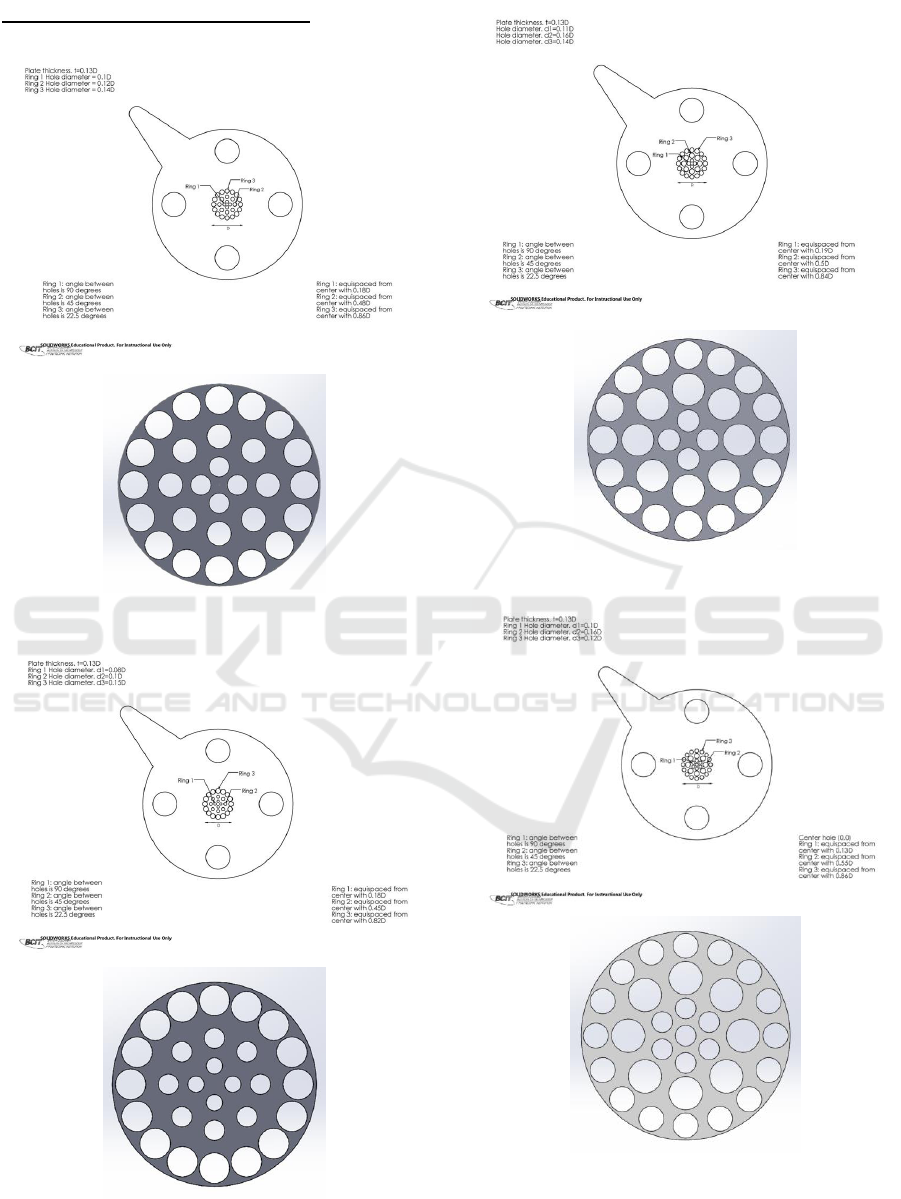
Flow Conditioner Design Drawings:

Design 1 Configuration (46.9% Porosity)

Design 2 Configuration (46.6% Porosity)

Design 3 Configuration (56.7% Porosity)

Design 4 Configuration (50.5% Porosity)

Computational Fluid Dynamics Model for Sensitivity Analysis and Design of Flow Conditioners

137

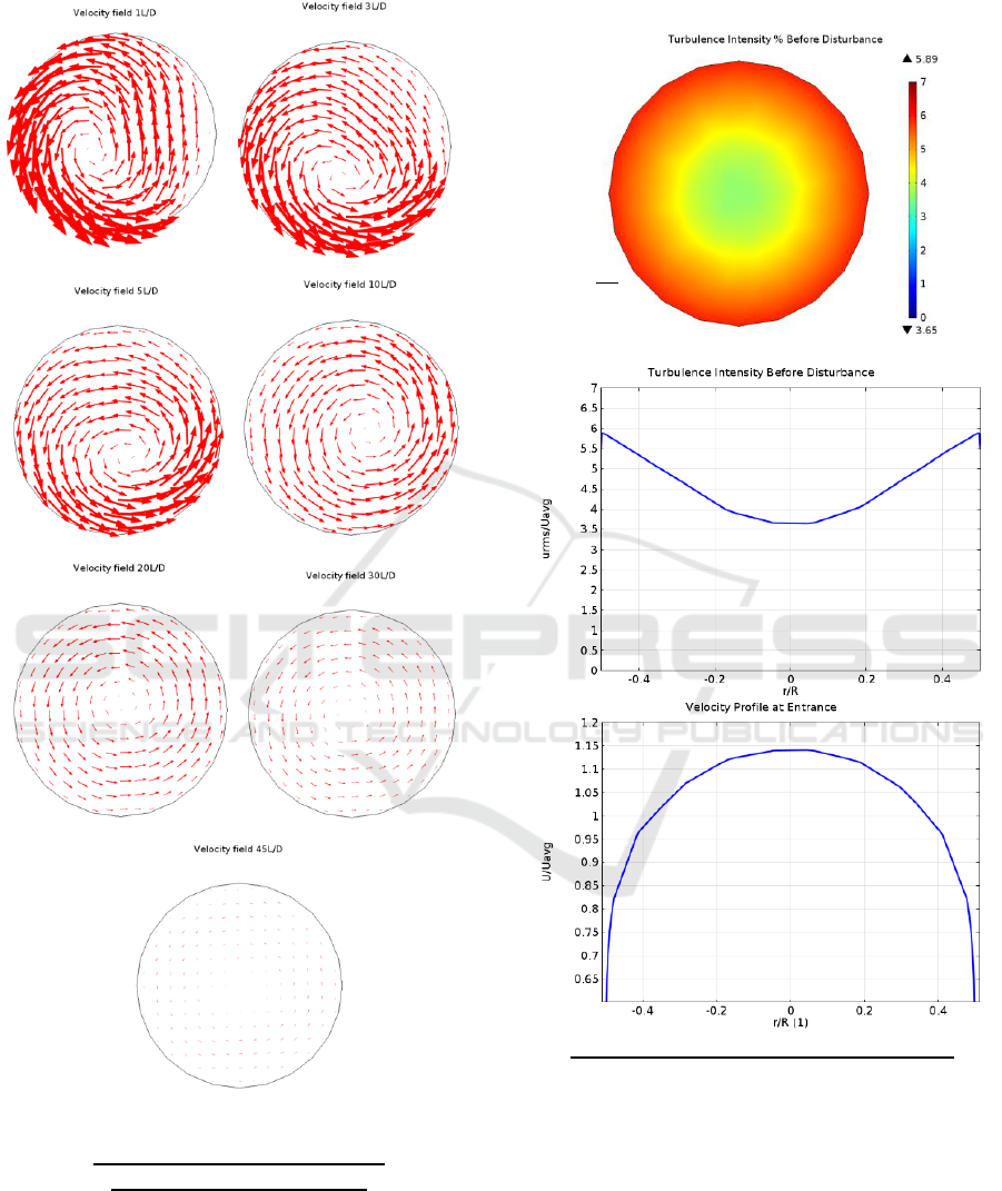
Out of plane Re=1.5E5 Double Elbow

Double out of plane 90 elbows

(Without flow conditioner)

Inlet Condition

Re=5E5

Flow condition upstream of Disturbance

 









SIMULTECH 2019 - 9th International Conference on Simulation and Modeling Methodologies, Technologies and Applications

138

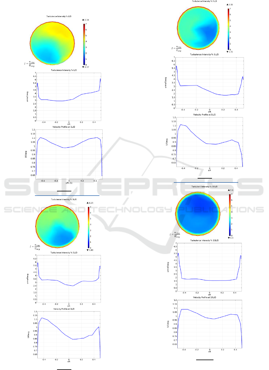
No Flow Conditioner Out of Plane Elbows

Re=1.5E5

1 L/D

3 L/D

5 L/D

10 L/D

Computational Fluid Dynamics Model for Sensitivity Analysis and Design of Flow Conditioners

139

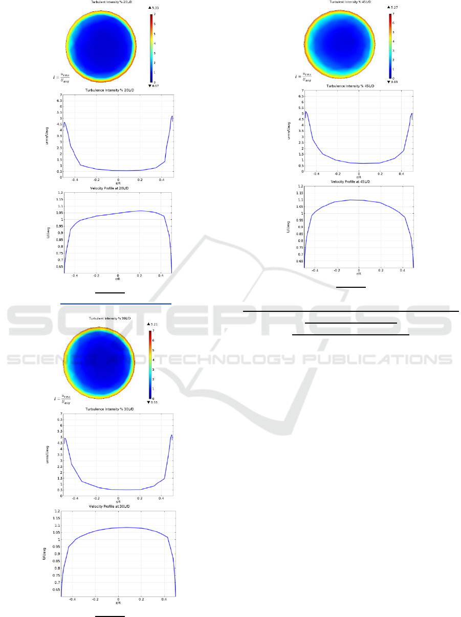
20 L/D

30 L/D

45 L/D

Double out of plane 90 elbows Velocity Profile &

Turbulence Intensity

(Without flow conditioner)

SIMULTECH 2019 - 9th International Conference on Simulation and Modeling Methodologies, Technologies and Applications

140