Estimating TCP Congestion Control Algorithms from Passively
Collected Packet Traces using Recurrent Neural Network
Naoki Ohzeki, Ryo Yamamoto, Satoshi Ohzahata and Toshihiko Kato
Graduate School of Informatics and Engineering, University of Electro-Communications,
1-5-1, Chofugaoka, Chofu, Tokyo 182-8585, Japan
Keywords: Tcp, Congestion Control, Passive Monitoring, Congestion Window, Recurrent Neural Network.
Abstract: Recently, as various types of networks are introduced, a number of TCP congestion control algorithms have
been adopted. Since the TCP congestion control algorithms affect traffic characteristics in the Internet, it is
important for network operators to analyse which algorithms are used widely in their backbone networks. In
such an analysis, a lot of TCP flows need to be handled and so the automatically processing is indispensable.
Thin paper proposes a machine learning based method for estimating TCP congestion control algorithms. The
proposed method uses a passively collected packet traces including both data and ACK segments, and
calculates a time sequence of congestion window size for individual TCP flows contained in the trances. We
use s recurrent neural network based classifier in the congestion control algorithm estimation. As the results
of applying the proposed classifier to ten congestion control algorithms, the major three algorithms were
clearly classified from the packet traces, and ten algorithms could be categorized into several groups which
have similar characteristics.
1 INTRODUCTION
Recently, along with the introduction of various types
of networks, such as a long-haul high speed network
and a wireless mobile network, a number of TCP
congestion control algorithms are designed,
implemented, and widely spread (Afanasyev et al.,
2010). Since the congestion control was introduced
(Jacobson, 1988), a few algorithms, such as TCP
Tahoe (Stevens, 1997), TCP Reno (Stevens, 1997),
and NewReno (Floyd et al., 2004), have been used
commonly for some decades. Recently, new
algorithms have been introduced and deployed. For
example, HighSpeed TCP (Floyd, 2003), Scalable
TCP (Kelly, 2003), BIC TCP (Xu et al., 2004),
CUBIC TCP (Ha et al., 2008), and Hamilton TCP
(Leith and Shorten, 2004) are designed for high speed
and long delay networks. TCP Westwood+ (Grieco
and Mascolo, 2004) is designed for lossy wireless
links. While those algorithms are based on packet
losses, TCP Vegas (Brakmo and Perterson, 2004)
triggers congestion control against an increase of
round-trip time (RTT). TCP Veno (Fu and Liew,
2003) combines loss based and delay based
approaches in such a way that congestion control is
triggered by packet losses but the delay determines
how to grow congestion window (cwnd). In 2016,
Google proposed a new algorithm called TCP BBR
(Cardwell et al., 2016) to solve problems mentioned
by conventional algorithms.
Since TCP traffic is a majority in the Internet
traffic and the TCP congestion control algorithms
characterize the behaviors of individual flows, the
estimation of congestion control algorithms for TCP
traffic is important for network operators. It can be
used in various purposes such as the traffic trend
estimation, the planning of Internet backbone links,
and the detection of malicious flows violating
congestion control algorithms.
The approaches for congestion control algorithm
estimation are categorized into the passive approach
and the active approach. The former estimates
algorithms from packet traces passively collected in
the middle of network by network operators. In the
latter approach, a test system communicates with a
target system with a specially designed test sequence
in order to identify the algorithm used in the target
system. Although the active approach is capable to
identify various congestion control algorithms
proposed so far, this approach does not fit the
algorithm estimation of real TCP flows by network
operators. On the other hand, the passive approaches
Ohzeki, N., Yamamoto, R., Ohzahata, S. and Kato, T.
Estimating TCP Congestion Control Algorithms from Passively Collected Packet Traces using Recurrent Neural Network.
DOI: 10.5220/0007916200270036
In Proceedings of the 16th International Joint Conference on e-Business and Telecommunications (ICETE 2019), pages 27-36
ISBN: 978-989-758-378-0
Copyright
c
 2019 by SCITEPRESS – Science and Technology Publications, Lda. All rights reserved
27

other than ours cannot estimate recently introduced
congestion control algorithms.
Previously, we proposed a passive method for
estimating congestion control algorithms (Kato et al.,
2014), (Kato et al., 2015). In this proposal, we
focused on the relationship between the estimated
congestion window sizes and their increments. The
relationship is indicated as a graph and the congestion
control algorithm is estimated based on the shape of
the graph. Our proposal succeeded to identify eight
congestion control algorithms implemented in the
Linux operating system, including recently
introduced ones.
However, the identification is performed
manually by human inspectors, and so it is difficult to
deal with a large number of TCP flows. This paper
proposes a new method for estimating congestion
control algorithms automatically based on the
machine learning. We estimate cwnd from packet
traces including both data and ACK segments, adopt
the recurrent neural network (RNN) as a machine
learning technique classifier, and show the results of
applying normalized cwnd time sequence to an RNN
classifier. We pick up ten congestion control
algorithms mentioned above and show how those
algorithms can be estimated automatically.
The rest of this paper is organized as follows.
Section 2 gives some background information
including the conventional studies on the congestion
control estimation and the machine learning applied
for the network areas. Section 3 describes the
proposed method and Section 4 gives the
performance evaluation results. In the end, Section 5
concludes this paper.
2 BACKGROUNDS
2.1 Studies on TCP Congestion Control
Algorithm Estimation
The proposals on the passive approach in the early
stage (Paxson, 1997), (Kato et al., 1997), (Jaiswel et
al., 2004) estimate the internal state and variables,
such as cwnd and ssthresh (slow start threshold), in a
TCP sender from bidirectional packet traces. They
emulate the TCP sender’s behavior from the
estimated state/variables according to the predefined
TCP state machine. But, they considered only TCP
Tahoe, Reno and New Reno and did not handle any
of recently introduced algorithms. (Oshio et al., 2009)
proposed a method to discriminate one out of two
different TCP congestion control algorithms
randomly selected from fourteen algorithms
implemented in the Linux operating system. This
method keeps track of changes of cwnd from a packet
trace and to extract several characteristics, such as the
ratio of cwnd being incremented by one packet.
Although this method targets all of the modern
congestion control algorithms, they assumed that the
discriminator knows two algorithms contained in the
packet trace.
Prior to our previous proposal, the only study
which can identify the TCP congestion control
algorithms including those introduced recently was a
work by (Yang et al., 2011). It is an active approach.
It makes a web server send 512 data segments under
the controlled network environment, and observes the
number of data segments contiguously transmitted.
From those results, it estimates the window growth
function and the decrease parameter to determine the
congestion control algorithm.
Our previous proposals (Kato et al., 2014), (Kato
et al., 2015) estimated cwnd in RTT intervals from
bidirectional packet traces, in the similar way with the
other methods. Different from other methods, we
focused on the incrementing situation of estimated
cwnd values. From the definition of individual
congestion control algorithms, the graph of cwnd
increments vs. cwnd has their characteristic forms.
For example, in the case of TCP Reno, the cwnd
increment is always one segment. In the case of
CUBIC TCP, the graph of cwnd increment follows a
√



curve. In this way, we proposed a way to
discriminate eight congestion control algorithms in
the Linux operating system.
2.2 Studies on Application of Machine
Learning to TCP
Recently, the machine learning is applied to various
fields in network technology. Examples are the
management of self-organizing network (Klaine,
2017), the intrusion detection (Buczak and Guven,
2016), and the identification of mobile applications
from network logs (Nakao and Du, 2018).
In the field of TCP, there are some studies on
applying machine learning published. (Edalat et al.,
2016) proposes a method to estimate RTT using the
fixed-share approach from measured RTT samples.
(Mirza et al., 2010) estimates the future throughput of
TCP flow using the support vector regression from
measured available bandwidth, queueing delay, and
packet loss rate. (Chung et al., 2017) proposes a
machine learning based multipath TCP scheduler
based on the radio strength in wireless LAN level,
wireless LAN data rate, TCP throughput, and RTT
with access point, by the random decision forests.
DCNET 2019 - 10th International Conference on Data Communication Networking
28

These proposals focused on the control aspects of
TCP. As far as we know, no attempts for the
congestion control algorithm estimation based on the
machine learning are not reported.
3 PROPOSED METHOD
3.1 Estimation of cwnd Values at RTT
Intervals
In the passive approach, packet traces are collected at
some monitoring point inside a network. So, the time
associated with a packet is not the exact time when
the node focused sends/receives the packet. Our
scheme adopts the following approach to estimate
cwnd values at RTT intervals using the TCP time
stamp option.
 Pick up an ACK segment in a packet trace. Denote
this ACK segment by ACK1.
 Search for the data segment whose TSecr (time
stamp echo reply) is equal to TSval (time stamp
value) of ACK1. Denote this data segment by
Data1.
 Search for the ACK segment which acknowledges
Data1 for the first time. Denote this ACK segment
by ACK2. Denote the ACK segment prior to
ACK2 by ACK1’.
 Search for the data segment whose TSecr is equal
to TSval of ACK2. Denote this data segment by
Data2.
From this result, we estimate a cwnd value at the
timing of receiving ACK1 as in (1).
 




(segments)
(1)

Here, seq means the sequence number, ack means the
acknowledgment number of TCP header, and MSS is
the maximum segment size.



is the truncation of a.
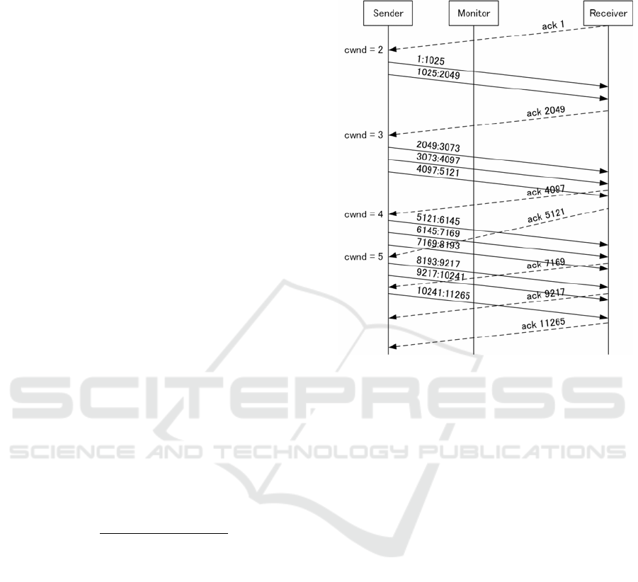
Figure 1 shows an example of cwnd estimation. In
this figure, the maximum segment size (MSS) is 1024
byte. Data segments are indicated by solid lines with
sequence number: sequence number + MSS. ACK
segments are indicated by dash lines with
acknowledgment number. When “ack 1” is picked up,
data segment “1:1024” is focused on as Data1 above.
ACK segment “ack 2049” responding the data
segment corresponds to ACK2. The ACK segment
before this ACK segment (ACK1’ above) is “ack 1”
again. Data2 in this case is “2049:3073.” So, the
estimated cwnd is (2049 – 1)/1024 = 2. Similarly, for
the following two RTT intervals, the estimated RTT
values are (5121 – 2049)/1024 = 3 and (10241 –5121)
/1024= 5.
Figure 1: Example of cwnd estimation.
3.2 Selection and Normalisation of
Input Data to Classifier
When a packet is lost and retransmitted, cwnd is
decreased. In order to focus on the cwnd handling in
the congestion avoidance phase, we select a time
sequence of cwnd between packet losses. We look for
a part of packet trace where the sequence number in
the TCP header keeps increasing. We call this
duration without any packet losses non-loss duration.
We use the time variation of estimated cwnd values
during one non-loss duration as an input to the
classifier.
However, the length of non-loss duration differs
for each duration, and the range of cwnd values in a
non-loss duration also differs from one to another. So,
we select and normalize the time scale and the cwnd
value scale for one non-loss duration.
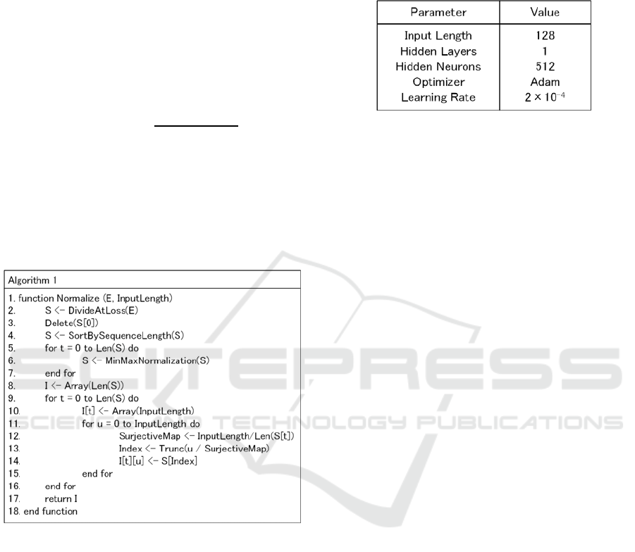
The algorithm for selecting and normalizing input
to classifier is given in Figure 2. In this algorithm, the
input E is as time sequence of cwnd values estimated
from one packet trace. The input InputLength is a
number of samples in one input to the classifier. In
this paper, we used 128 as InputLength.
In the beginning, the time sequence of cwnd is
divided at packet losses, and the divided sequences
are stored in a two dimensional array S. Next, the first
Estimating TCP Congestion Control Algorithms from Passively Collected Packet Traces using Recurrent Neural Network
29

sequence S[0] is removed, because we focus only on
the congestion avoidance phase. Then S is reordered
according to the length of cwnd sequence. Then the
cwnd values for one sequence S[t] are normalized
between 0 and 1. The normalization is performed in
the following way.
Let 




max






for 0⋯Len





1, and





min






for 0⋯Len





1.
Each cwnd value in S[t] is normalized by






←

















.
After that, the cwnd values are resampled into the
number of InputLength (128 in this paper). This is
done by the loop between step 11 and step 15. As a
result, a cwnd sequence in S[t] is converted to an array
I[t] with 128 elements. By this algorithm, all of the
time sequences of cwnd values are the arrays with 128
elements whose value is between 0 and 1.
Figure 2: Selection/normalization algorithm.
3.3 RNN based Classifier for
Congestion Control Algorithm
Estimation
We used RNN for constructing the classifier, whose
output layer defines the TCP congestion control
algorithms. The neural network is widely used for the
classification, regression, and estimation for various
data. Especially, RNN is designed for handling
temporal ordered behaviors, including video/speech
recognition and handwriting recognition. Since we
deal with the time sequence of cwnd values, RNN is
considered to be appropriate for our classifier.
Among the RNN technologies, we pick up the long
short-term memory mechanism (Hochreiter and
Schmidhuber, 1997), which was proposed to handle a
relatively long time sequence of data.
Table 1: Hyper parameters of classifier.
The input is a normalized time sequence of cwnd
as described above, with using labels of congestion
control algorithms represented by one-hot vector. The
hyper parameters of RNN is defined as shown in
Table 1. Here, we used relatively large number of
hidden neurons in order to install strong
representation capability in the hidden layer.
Specifically, the number of hidden neuron is 512
while the input length is 128.
In the training of the classifier, we use the mini-
batch method, which selects a specified number of
inputs randomly from the prepared training data. The
mini-batch size will be determined for individual
training. The training will be continued until the result
of the loss function becomes smaller than the learning
rate.
4 EXPERIMENT RESULTS
4.1 Experimental Setup
Figure 3 shows the experimental configuration for
collecting time sequence of cwnd values. A data
sender, a data receiver, and a bridge are connected via
100 Mbps Ethernet links. In the bridge, 50 msec delay
for each direction is inserted. As a result, the RTT
value between the sender and the receiver is 100 msec.
In order to generate packet losses that will invoke the
congestion control algorithm, packet losses are
inserted randomly at the bridge. The average packet
loss ratio is 0.01%. The data transfer is performed by
use of iperf3 (iPerf3, 2019), executed in both the
sender and the receiver. The packet traces are
collected by use of tcpdump at the sender’s Ethernet
interface. We use the Python 3 dpkt module (dpkt,
2019) for the packet trace analysis. We changed the
congestion control algorithm at the receiver by use of
the sysctl command provided by the Linux operating
system.
DCNET 2019 - 10th International Conference on Data Communication Networking
30

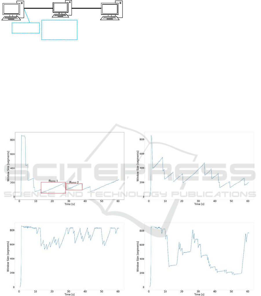
Figure 3: Experiment configuration.
4.2 Results of cwnd Estimation from
Packet Traces and Normalization
We used TCP Reno, HighSpeed TCP, Scalable TCP,
BIC TCP, CUBIC TCP, Hamilton TCP, TCP
Westwood+, TCP Vegas, TCP Veno, and TCP BBR,
at the sender. Figures 4 through 13 are examples of
time sequence of estimated cwnd values. In those
example, the data transfer by iperf3 is performed for
60 sec. The cwnd values are estimated in terms of
segment according to the method described in
Subsection 3.1. It can be recognized that the time
variation of cwnd values present characteristical
shapes representing individual algorithms, but it may
be difficult to estimate algorithms manually. So, we
apply the RNN machine learning method to those
results.
As described in Subsection 3.2, a part of cwnd
sequences in duration when there are no
retransmissions is handled as a separate input
sequence. Figures 4 and 8 gives examples of such
sequences, indicated as Reno 1, Reno 2, CUBIC 1,
and CUBIC 2. As shown by these examples, the size
of these sequences differ from each other, both for the
time scale and the scale of cwnd. Therefore, it is
necessary for normalize these sequence. Figure 14
illustrate how these sequences are normalized.
Different scale of cwnd time sequences are
transformed into a canonical form with 128 samples
in the range of 0 through 1.
Figure 4: Estimated cwnd for TCP Reno. Figure 5: Estimated cwnd for HighSpeed TCP.
Figure 6: Estimated cwnd for Scalable TCP. Figure 7: Estimated cwnd for BIC TCP.
Sender Receiver
100 Mbps
Ethernet
Bridge
inserting
100msec RTT
and 0.01%
packet error
100 Mbps
Ethernet
capturing
packets
Estimating TCP Congestion Control Algorithms from Passively Collected Packet Traces using Recurrent Neural Network
31

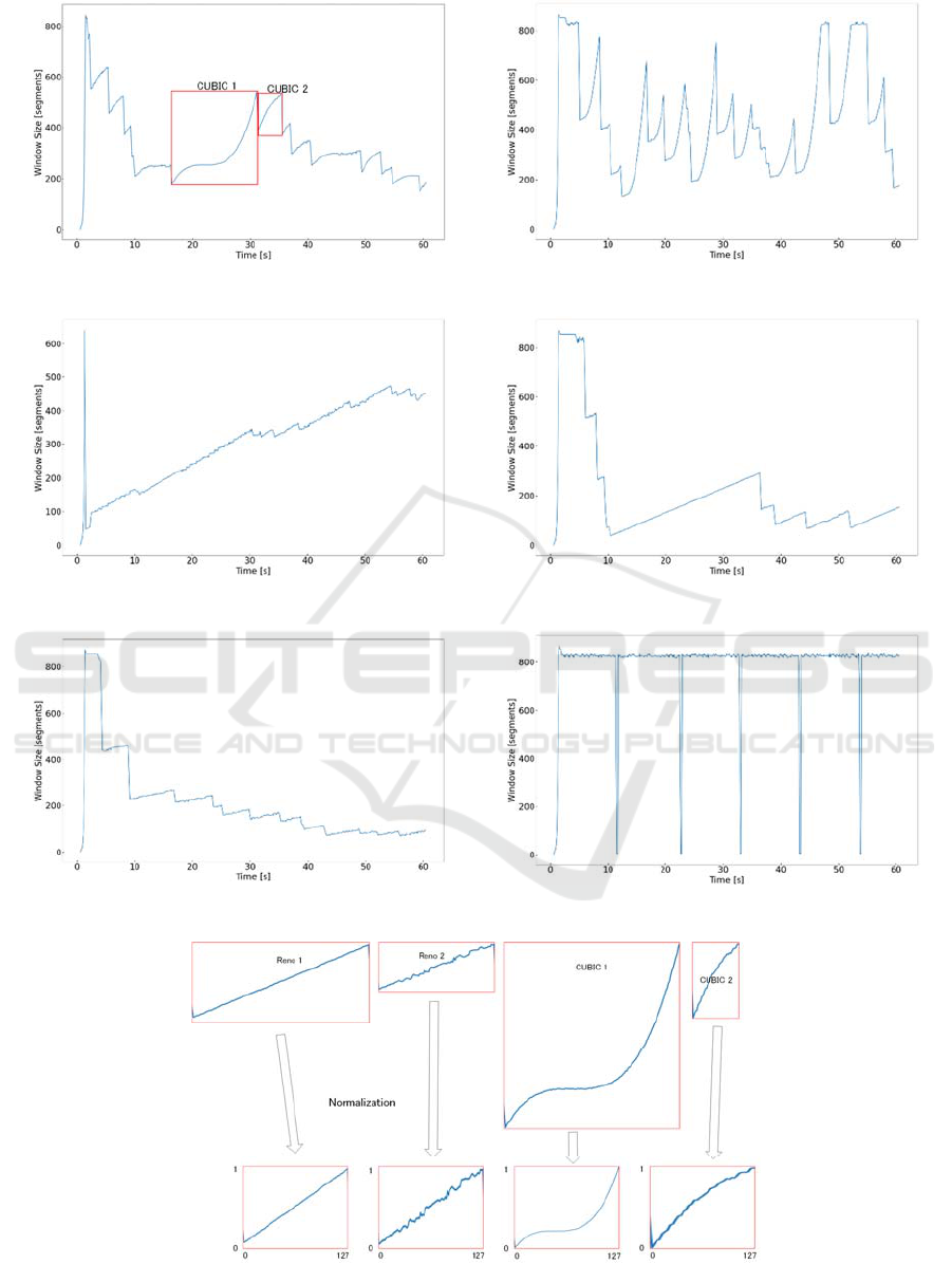
Figure 8: Estimated cwnd for CUBIC TCP. Figure 9: Estimated cwnd for Hamilton TCP.
Figure 10: Estimated cwnd for TCP Westwood+. Figure 11: Estimated cwnd for TCP Vegas.
Figure 12: Estimated cwnd for TCP Veno.
Figure 13: Estimated cwnd for TCP BBR.
Figure 14: Example of normalization.
DCNET 2019 - 10th International Conference on Data Communication Networking
32

4.3 Results of Congestion Control
Algorithm Estimation
4.3.1 Overview of Classifier
We implemented the classifier for the TCP
congestion control algorithms by the TensorFlow
library (TensorFlow, 2019) supported by Google.
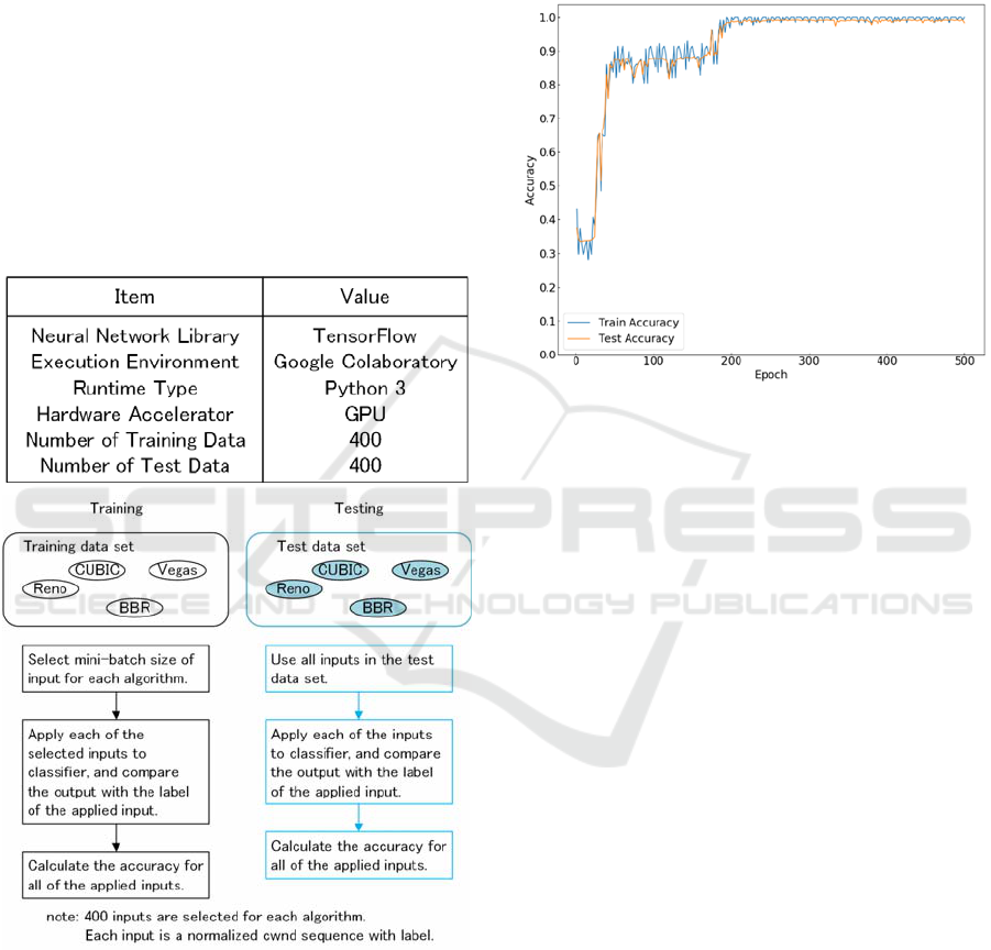
Table 2 shows the environment for machine learning.
The program language we used for TensorFlow is
Python 3, and the execution environment is the
Google Colaboratory tool (Google Colab, 2019). It
allows to use GPU over the Google cloud platform.
We prepared 400 test inputs for individual congestion
control algorithms both as training data and test data.
Table 2: Environment for machine learning.
Figure 15: Overview of experiment.
Figure 15 shows an overview of our experiment.
First, we performed ten minute data transfer using
iperf3 ten times for producing training data and test
data, respectively. From those packet traces, we
collected cwnd time sequences for non-loss durations,
excluding the first ones in individual iperf3 runs.
After that, we sorted the obtained cwnd time
sequences according to the number of samples. Those
steps were done for individual congestion algorithms.
From those sets of sorted cwnd time sequences, we
selected top 400 samples for training data and test
data, for individual algorithms, and performed the
normalization. These results are shown as two round
corner rectangles in the top of Figure 15.
Figure 16: Learning curve for three algorithms.
Then, we executed training and test alternatively
in each trial. As for the training, we select the mini-
batch size of inputs for individual congestion control
algorithm. We apply the selected training inputs to the
classifier and check whether the output of the
classifier matches the label of input. We collect all the
results for all training inputs and calculate the
accuracy for individual congestion control algorithms.
Then we move to the testing. In the testing, we use
all of 400 inputs for individual congestion control
algorithms. We apply all test inputs to the classifier
and compare the classifier output and the label of
inputs. From those results, we calculate the accuracy
for test data.
We go to next epoch, and perform the training
phase and the test phase. In the training phase, we
select another set of training data, and we use all
inputs in the test data again. We continue this
experiment until the return value of the loss function
becomes the learning rate.
4.3.2 Results for Major Three Congestion
Control Algorithms
As the first experiment, we focused on TCP Reno,
CUBIC TCP, and TCP BBR. The reason we select
these three algorithms is as follows. TCP Reno has
been used widely since the congestion control was
introduced. CUBIC TCP is the default algorithm in
major operating systems including Windows, mac OS,
Estimating TCP Congestion Control Algorithms from Passively Collected Packet Traces using Recurrent Neural Network
33

and Linux as of writhing this paper. TCP BBR is a
new version proposed by Google, in order to resolve
the problems the conventional congestion control
algorithms suffer from.
In this experiment, we used the mini-batch size of
128. Figure 16 shows the learning curve for these
three algorithms. The horizontal axis of this figure
shows the epoch, the number of training and test trials.
The vertical axis shows the accuracy for the training
process and the test process. The blue line is the
accuracy for the training process and the red line is
for the test process. The graphs in Figure 16 show that
both the training accuracy and the test accuracy are
converging to 1.0 as the epoch is increasing. This
means that there is no overtraining in the classifier.
1
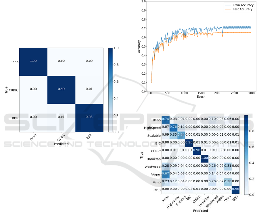
Figure 17: Confusion matrix for three algorithms.
Figure 17 shows the confusion matrix indicating
the result throughout this experiment. Each row
corresponds to the label of true value (Reno, CUBIC,
and BBR), and each column corresponds to the label
of predicted value. The results of the prediction are
indicated by looking at each column. TCP Reno is
identified at the accuracy of 1.0. CUBIC TCP is
identified at the accuracy of 0.98, and the ratio of 0.1
is mis-identified as TCP BBR. TCP BBR is identified
at the accuracy of 0.98, and mis-identified as CUBIC
TCP at the ratio of 1.0. These results say that the
estimation of three congestion control method is well
performed by the RNN based classifier.
4.3.3 Results for Ten Congestion Control
Algorithms
As the second experiment, we conducted the
congestion control algorithm estimation for ten
algorithms listed in Subsection 4.2. In this experiment,
we used 256 as a mini-batch size. Figure 18 shows the
learning curve for ten congestion control algorithms.
Similarly with Figure 16, the horizontal axis is the
epoch and the vertical axis is the accuracy. The blue
line in the graph is for the training process and the red
line is for the test process. Here, for the epoch which
is 2,200 and later, the accuracy for the training
process is stable around 0.7, and that for the test
process is around 0.65.
Figure 18: Learning curve for ten algorithms.
Figure 19: Confusion matrix for ten algorithms.
Figure 19 shows the confusion matrix for this
experiment. Among ten congestion control
algorithms, BIC TCP, CUBIC TCP, Hamilton TCP,
and TCP BBR are uniquely identified. HighSpeed
TCP and Scalable TCP are predicted confusingly.
The reason may be that the congestion avoidance
behaivors of these two algorithms were similar with
each other in our experiment condition. Considering
that these two algorithms are early stage aggressive
algorithms intended for high speed long haul
networks, this result may be reasonable.
DCNET 2019 - 10th International Conference on Data Communication Networking
34

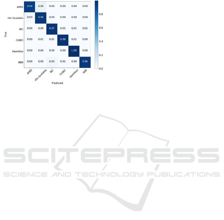
Figure 20: Confusion matrix for grouped algorithms.
As for TCP Reno, Westwood+, TCP Vegas, and
TCP Veno, those algorithms are based on the additive
increase multiplicative decrease (AIMD) principle in
the congestion avoidance phase. Westwood+ differs
from the TCP Reno in the behavior of cwnd shrinking.
But in our experiment, only the cwnd increasing
behavior is focused on. TCP Vegas and TCP Veno
differ from TCP Reno in the behavior when the RTT
is increasing due to the congestion. But in our
experiment, the congestion is invoked by the artificial
impairment, i.e., inserted packet losses, and so the
situation when RTT is increasing is not considered.
Therefore, the result that these four algorithms are
mis-identified is resulting from the characteristic of
training data in our experiment.
Figure 20 shows the confusion matrix in which we
grouped TCP Reno, Westwood+, TCP Vegas, and
TCP Veno into one category named AIMD, and
HighSpeed TCP and Scalable TCP into one category.
Each category is identified correctly in this result.
5 CONCLUSIONS
In this paper, we showed a result of TCP congestion
control algorithm estimation using a recurrent neural
network. From packet traces including both data
segments and ACK segments, we derived a time
sequence of cwnd values at RTT intervals without
any packet retransmissions. By ordering the time
sequences and normalizing in the time dimension and
the cwnd value dimension, we obtained the input for
the RNN classifier. As the results of applying the
proposed classifier for ten congestion control
algorithms implemented in the Linux operating
system, the major three algorithms, TCP Reno,
CUBIC TCP, and BBR, were clearly classified from
each other, and ten algorithms could be categorized
into several groups which have similar
characteristics.
REFERENCES
Afanasyev, A., Tilley, N., Reiher, P., Kleinrock, L., 2010.
Host-to-Host Congestion Control for TCP. IEEE
Commun. Surveys & Tutorials, vol. 12, no. 3, pp. 304-
342.
Jacobson, V., 1988. Congestion Avoidance and Control.
ACM SIGCOMM Comp. Commun. Review, vol. 18, no.
4, pp. 314-329.
Stevens, W. R., 1997. TCP Slow Start, Congestion
Avoidance, Fast Retransmit, and Fast Recovery
Algotithms. IETF RFC 2001.
Floyd, S., Henderson, T., Gurtov, A., 2004. The NewReno
Modification to TCP’s Fast Recovery Algorithm. IETF
RFC 3728.
Floyd, S., 2003. HighSpeed TCP for Large Congestion
Windows. IETF RFC 3649.
Kelly, T., 2003. Scalable TCP: Improving Performance in
High-speed Wide Area Networks. ACM SIGCOMM
Comp. Commun. Review, vol. 33, no. 2, pp. 83-91.
Xu, L., Harfoush, K., Rhee, I., 2004. Binary increase
congestion control (BIC) for fast long-distance
networks. In Proc. IEEE INFOCOM 2004, vol. 4, pp.
2514-2524.
Ha, S., Rhee, I., Xu, L., 2008. CUBIC: A New TCP-
Friendly High-Speed TCP Variant. ACM SIGOPS
Operating Systems Review, vol. 42, no. 5, pp. 64-74.
Leith, D., Shorten, R., 2004. H-TCP: TCP for high-speed
and long distance networks. In Proc. Int. Workshop on
PFLDnet, pp. 1-16.
Grieco, L., Mascolo, S., 2004. Performance evaluation and
comparison of Westwood+, New Reno, and Vegas TCP
congestion control. ACM Computer Communication
Review, vol. 34, no. 2, pp. 25-38.
Brakmo, L., Perterson, L., 1995. TCP Vegas: End to End
Congestion Avoidance on a Global Internet. IEEE J.
Selected Areas in Commun., vol. 13, no. 8, pp. 1465-
1480.
Fu, C., Liew, S., 2003. TCP Veno: TCP Enhancement for
Transmission Over Wireless Access Networks. IEEE J.
Sel. Areas in Commun., vol. 21, no. 2, pp. 216-228.
Cardwell, N., Cheng, Y., Gumm, C. S., Yeganeh, S. H.,
Jacobson, V., 2016. BBR: Congestion-Based
Congestion Control. ACM Queue vol. 14 no. 5, pp. 20-
53.
Kato, T., Oda, A., Ayukawa, S., Wu, C., Ohzahata, S., 2014.
Inferring TCP Congestion Control Algorithms by
Correlating Congestion Window Sizes and their
Differences. In Proc. IARIA ICSNC 2014, pp.42-47.
Kato, T., Oda, A., Wu, C., Ohzahata, S., 2015. Comparing
TCP Congestion Control Algorithms Based on
Passively Collected Packet Traces. In Proc. IARIA
ICSNC 2015, pp. 145-151.
Estimating TCP Congestion Control Algorithms from Passively Collected Packet Traces using Recurrent Neural Network
35

Paxson, V., 1997. Automated Packet Trace Analysis of
TCP Implementations. ACM Comp. Commun. Review,
vol. 27, no. 4, pp.167-179.
Kato, T., Ogishi, T., Idoue, A., Suzuki, K., 1997. Design of
Protocol Monitor Emulating Behaviors of TCP/IP
Protocols. In Proc. IWTCS ’97, pp. 416-431.
Jaiswel, S., Iannaccone, G., Diot, C., Kurose, J., Towsley,
D., 2004. Inferring TCP Connection Characteristics
Through Passive Measurements. In Proc. INFOCOM
2004, pp. 1582-1592.
Oshio, J., Ata, S., Oka, I., 2009. Identification of Different
TCP Versions Based on Cluster Analysis. In Proc.
ICCCN 2009, pp. 1-6.
Qian, F., Gerber, A., Mao, Z., 2009. TCP Revisited: A
Fresh Look at TCP in the Wild. In Proc. IMC ’09, pp.
76-89.
Yang, P., Luo, W., Xu, L., Deogun, J., Lu, Y., 2011. TCP
Congestion Avoidance Algorithm Identification. In
Proc. ICDCS ’11, pp. 310-321.
Klaine, P., Imran, M., Onireti, O., Souza, R., 2017. A
Survey of Machine Learning Techniques Applied to
Self-Organizing Cellular Networks. IEEE Commun.
Surveys & Tutorials, vol. 19, no. 4, pp. 2392-2431.
Buczak A., Guven, E., 2016. A Survey of Data Mining and
Machine Learning Methods for Cyber Security
Intrusion Detection. IEEE Commun. Surveys &
Tutorials, vol. 18, no. 2, pp. 1153-1176.
Nakao, A., Du, P., 2018. Toward In-Network Deep
Machine Learning for Identifying Mobile Applications
and Enabling Application Specific Network Slicing.
IEICE Trans. Commun., vol. E101-B, no. 7, pp. 1536-
1543.
Edalat, Y., Ahn, J., Obraczka, K., 2016. Smart Experts for
Network State Estimation. IEEE Trans. Network and
Service Management, vol. 13, no. 3, pp. 622-635.
Mirza, M., Sommers, J., Barford, P., Zhu, X., 2010. A
Macine Learning Approach to TCP Throughput
Prediction. IEEE/ATM Trans. Networking, vol. 18, no.
4, pp. 1026-1039.
Chung, J., Han, D., Kim, J., Kim, C., 2017. Machine
Learning based Path Management for Mobile Devices
over MPTCP. In Proc. 2017 IEEE International
Conference on Big Data and Smart Computing
(BigComp 2017), pp. 206-209.
Hochreiter, S., Schimidhuber, J., 1997. Long short-term
memory. Neural Computation, vol. 9, no. 8, pp. 1735-
1780.
iPerf3, 2019. iPerf - The ultimate speed test tool for TCP,
UDP and SCTP. https://iperf.fr/.
dpkt, 2019. dpkt. https://dpkt.readthedocs.io/en/latest/.
TensorFlow, 2019. TensorFlow.
https://www.tensorflow.org/.
Google Colab, 2019. Google Colaboratory.
https://colab.researach.google.com/.
DCNET 2019 - 10th International Conference on Data Communication Networking
36