Entry Trajectory Optimization via hp
Pseudospectral Convex Programming
Xiao Wang
a
, Yulin Wang
b
, Shengjing Tang
c
and Jie Guo
d
School of Aerospace and Engineering, Beijing Institute of Technology, Beijing, China
Keywords: Entry Guidance, Trajectory Optimization, Convex Programming, Pseudospectral Method.
Abstract: In this paper, a hp pseudospectral sequential convex programming (hp-PSCP) method is proposed to solve
the entry trajectory optimization problem. The hp flipped Radau pseudospectral method (FRPM) is utilized
to discretize the nonlinear dynamics. By successive linearization technology and introducing new variables,
the optimization problem is converted into a series of convex problems and solved by primal-dual interior-
point method. Numerical results show that the proposed method provides a good compromise between
computational accuracy and speed compared to existing convex methods.
1 INTRODUCTION
Entry phase, which is from space to atmosphere, is
the key stage for the flight of entry vehicles, including
reusable launch vehicles and hypersonic gliding
vehicles. Entry guidance is always a difficult issue of
the research of entry vehicles (Lu, 2014). With the
development of onboard entry guidance,
requirements for online trajectory optimization
methods are increasing. Generally, trajectory
optimization methods can be divided into two groups:
direct methods and indirect methods (Betts, 1998).
Indirect methods use Pontryagin’s minimum
principle to transform optimal control problem into a
boundary-value problem. Indirect methods guarantee
the optimality of the solution, while the boundary-
value problem is hard to solve and sensitive to initial
guess. In contrast, direct methods discretize the
original optimal control problem into a parameter
optimization problem and solve the parameter
optimization problem by nonlinear programming
(NLP) algorithms. With the development of NLP
algorithms, large-scale NLP problems can be solved
precisely. However, the solving process is rather
time-consuming for complicated trajectory
optimization problems. Consequently, traditional
a
https://orcid.org/0000-0002-7583-7628
b
https://orcid.org/0000-0003-2666-836X
c
https://orcid.org/0000-0003-4224-9579
d
https://orcid.org/0000-0003-0951-5126
approaches may be not suitable for onboard
applications.
Recently, convex optimization has attracted wide
attention due to its application in aerospace guidance
and control, such as Mars powered landing
(Acikmese et al., 2005; Acikmese et al., 2007;
Blackmore et al., 2010), low-thrust orbit transfers
(Wang and Grant, 2017
1
), spacecraft rendezvous (Lu
and Liu, 2013), path planning for unmanned aerial
vehicles (Wang and Liu, 2017) and constrained
missile guidance (Liu et al., 2016). Convex
optimization can be divided into several subclasses,
including linear programming (LP), quadratic
programming (QP), second-order cone programming
(SOCP), and semidefinite programming (SDP). If the
optimization problem is formulated as one of them, it
can be solved in polynomial time (Boyd et al., 2004).
Mature primal-dual interior-point method (IPM) has
been investigated to solve the convex optimization
problem (Wright, 1997). With IPM, the globally
optimal solution can be found in a number of
iterations with deterministic upper bound. Besides,
initial guesses are not required in IPM. With these
advantages, convex optimization is a very promising
approach for onboard trajectory optimization.
However, highly nonlinear dynamics and constraints
are the main difficulties for the application of convex
Wang, X., Wang, Y., Tang, S. and Guo, J.
Entry Trajectory Optimization via hp Pseudospectral Convex Programming.
DOI: 10.5220/0007909800610069
In Proceedings of the 16th International Conference on Informatics in Control, Automation and Robotics (ICINCO 2019), pages 61-69
ISBN: 978-989-758-380-3
Copyright
c
 2019 by SCITEPRESS – Science and Technology Publications, Lda. All rights reserved
61

optimization. A SOCP method was developed for
entry trajectory optimization problem where the
dynamics equations with respect to the variable of
energy were used (Liu et al., 2015
1
). The original
dynamics was relaxed into a SOCP form via
successive linearization. On the base of this work, the
smooth entry problem and maximum-crossrange
entry problem were investigated using similar way
(Liu et al., 2015
2
; Liu and Shen, 2016). Distinguish
from (Liu et al., 2015
1
), a sequential convex
programming (SCP) algorithm was designed (Wang
and Grant, 2017
2
), where the original dynamics with
respect to time were used and the rate of bank angle
was extended to a new control variable. Then this
algorithm was used to design an autonomous entry
guidance method (Wang and Grant, 2018).
The approaches mentioned above employ
trapezoidal rule with uniform distributions of nodes
as the discretization method, leading to low
discretization precision (Sagliano, 2017). Moreover,
only fixed-flight-time problem is considered, and the
final flight time cannot be optimized, which is
obviously not suitable for practical flight.
Pseudospectral (PS) method, which discretizes the
state and control variables on orthogonal collocation
points, may be an alternative approach for entry
trajectory optimization (Fahroo and Ross, 2008). The
state and control variables are approximated by global
Lagrange interpolations, resulting in higher
discretization precision and smoother results. The
total time domain is transformed to [−1,1], making PS
method suitable for free-time problem. To solve
powered landing problems, convex optimization has
been combined with PS method. Acikmese et al.
firstly used Chebyshev polynomials to interpolate the
controls (Acikmese et al., 2005). Sagliano proposed
the pseudospectral convex optimization for powered
descent guidance with more precise results than
standard convex methods (Sagliano, 2017; Sagliano,
2018). The pseudospectral sequential convex
optimization is embedded into the model predictive
control framework for rocket vertical landing
guidance (Wang et al., 2019).
However, in standard PS method, the state
variable on each node is associated with all state
variables, since the Lagrange interpolation is a global
interpolation method, leading to a less sparse
structure of the underlying matrices. Thus the CPU
time after discretization is quite longer than other
methods, such as Euler method and trapezoidal rule.
In this paper, the hp PS method and the sequential
convex programming are united in one framework to
alleviate this effect for the entry trajectory
optimization problem. In hp PS method, which has
been implemented successfully in other optimization
packages (Patterson and Rao, 2014), the whole time
domain is broken into several subdomains and the
state variable is only associated with the state
variables of each subdomain. Therefore, compared
with standard PS method, faster results with similar
accuracy can be obtained.
This paper is organized as follows: In Section 2,
the entry trajectory optimization problem is
described. Section 3 presents the whole hp
pseudospectral sequential convex programming (hp-
PSCP) method. The numerical results are shown in
Section 4 and the work is summarized in Section 5.
2 PROBLEM FORMULATION
In this section, we formulate the optimal control
problem derived from the entry trajectory
optimization problem.
2.1 Entry Dynamics
This paper considers Earth as a non-rotating spherical
model. Instead of the energy-based equations for
entry vehicles, we use the original equations of
motion. The dimensionless three degree of freedom
equations of motion of an entry vehicle are (Lu, 2014)
2
2
2
sin
cos sin / ( cos )
cos cos /
sin /
cos / ( 1/ ) cos / ( )
sin / ( cos ) cos sin tan /
rV
Vr
Vr
VD r
LVVr Vr
L
VV r




 

 









 













(1)
where
r
is the dimensionless radius from the Earth
center to the vehicle, which is normalized by
0
6371kmR

.

and

denotes the longitude and
latitude, respectively. V denotes the dimensionless
flight velocity, which is normalized by
00
g
R with
2
0
9.81m/sg 
.

denotes the flight path angle and

denotes the heading angle.

is the bank angle.
The dimensionless time t in the differentiation of the
equations (1) is normalized by
00
/Rg. L and D
denote the dimensionless lift and drag accelerations,
respectively, which is normalized by
0
g
.
ICINCO 2019 - 16th International Conference on Informatics in Control, Automation and Robotics
62

2
0
2
0
(,) /(2)
(,) /(2)
Lref
Dref
LRVC VS m
DRVC VS m









(2)
where m is the mass,
ref
S
is the reference area,
L
C
and
D
C are the lift and drag coefficients, respectively,
which are functions of angle of attack

and velocity,

is the atmospheric density calculated by

0
/
0
hh
he 


(3)
where
h
is the altitude,
0

is the atmospheric density
at sea level and
0
h is an altitude constant.
In this paper, the angle of attack

is assumed as
a function of velocity. The bank angle

is the only
control variable for trajectory optimization.
Furthermore, following the way in [16], we choose
the bank angle rate,


, as the new control variable to
constrain the change rate of bank angle and eliminate
the potential high-frequency oscillations, that is,
u



(4)
where u is new control variable. By adding equations
(4) to the original equations of motion (1), the
augmented equations of motion can be transformed
into an affine form:
() Bu

xfx
(5)
where
[;;;;;;]rV

 x
is state vector with seven
elements. The function
()fx and matrix B are given
by
2
2
2
sin
cos sin / ( cos )
cos cos /
() sin /
cos / ( 1/ ) cos / ( )
sin / ( cos ) cos sin tan /
0
V
Vr
Vr
Dr
LVVr Vr
L
VV r

 



 






 








fx
(6)
= [0;0;0;0;0;0;1]B
(7)
In this new model, the control variable is
decoupled from the sates, which will potentially
benefit the convergence of the follow-up hp-PSCP
algorithms.
2.2 Trajectory Optimization Problem
For an entry flight, the initial and terminal state
vectors are predefined:
00
() , ( )
f
f
tt

xxx x
(8)
where
0
x is the initial state and
f
x
is the given
terminal state.
0
t is the initial flight time and
f
t
is the
free final flight time. During the entry flight, both the
states and control are bounded:
min max
[, ]

xx x
(9)
max
uu
(10)
where
max
u is the upper bound of the bank angle rate,
and
min max
,xx are the lower and upper bounds of the
states, respectively. Besides, the typical path
constraints, including heat rate, dynamic pressure and
normal load, are considered
0.5 3.15
maxQ
Qk V Q  

(11)
2
max
/2qV q  
(12)
22
max
nLDn
(13)
where
Q
k
is a constant, and
Q

,
q
,
n
are the heating
rate, the dynamic pressure and the normal load,
respectively.
max
Q

,
max
q
,
max
n
are the upper bounds
of them, respectively.
In this paper, a general cost function is considered
as follows:
0
[( )] (,)
f
t
f
t
J
tldt  

xxu
(14)
Based on above discussion, the entry trajectory
optimization can be defined as a nonlinear optimal
control problem as follows:
Problem 0:
Minimize: (14)
Subject to: (5), (8)-(13)
P0 is a free-time optimal control problem, and the
terminal flight time can be optimized (instead of fixed
offline) which is a significant difference from (Liu et
al., 2015
1
; Wang and Grant, 2017
2
) and more
accordant with practical flight.
Entry Trajectory Optimization via hp Pseudospectral Convex Programming
63

3 TRAJECTORY OPTIMIZATION
ALGORITHM
3.1 Flipped Radau Pseudospectral
Method
For solving optimal control problem, numerical
methods are usually divided into two classes: direct
methods and indirect methods. In direct methods, the
dynamics equations are discretized and the optimal
control problem is transformed into a finite
dimensional NLP problem. Among direct methods,
pseudospectral (PS) methods discretize the state and
control variables on orthogonal collocation points
simultaneously. PS methods have high discretization
precision and converge faster for smooth problems.
Among a variety of PS methods, in this paper, we
choose the flipped Radau pseudospectral method
(FRPM). It has been proved that FRPM owns a
smoother convergence with respect to other PS
methods.
FRPM is an asymmetric PS method. First, we
introduce the flipped Legendre-Gauss-Radau (LGR)
polynomial
1
() () () [1,1]
nnn
RLL



 
(15)
where
()
n
R

denotes the flipped Legendre-Gauss-
Radau polynomial of order n and
()
n
L

denotes the
Legendre polynomial of order n. n LGR points are
the roots of
()
n
R

on (−1,1] and are chosen as the
collocation nodes of FRPM. Besides, −1 is chosen as
the first discretization node. Then there are n+1
discretization nodes on [−1,1] in FRPM.
In FRPM, the state and control variables are
represented by orthogonal polynomials defined on
[−1, 1]. The time domain of the optimal control
problem is normalized by the affine transformation
0
00
2
f
ff
tt
t
tttt




(16)
The state and control variables are approximated
by Lagrange interpolations
01
() ( ) (), () ( ) ()
nn
ii ii
ii
PP

 



xx uu
(17)
where
()
i
P

and
()
i
P

are the Lagrange interpolation
polynomials. Though Lagrange interpolation, the
derivative of
()

x can be approximated by the linear
summation of
()
i

x . Then the flipped Radau
pseudospectral differentiation matrix D is introduced
(Patterson and Rao, 2014).
0
()
( ), 1,...,
n
k
ki i
i
d
kn
d






x
Dx
(18)
At n LGR points, the dynamics equations are
transformed into algebraic constraints by using (18)
0
0
( ) [ ( ), ( )] 0, 1,...,
2
n
f
ki i k k
i
tt
kn





Dx Fx u
(19)
where
(,)F xu is the right-hand side of the dynamics
equation.
Similarly, the cost function (14) can be replaced
by
0
1
[ ( ), ( )]
2
[(1)]
n
f
kkk
k
tt
wlJ






xxu
(20)
where
k
w is the corresponding weight at the LGR
points.
3.2 hp Flipped Radau Pseudospectral
Method
In the basic FRPM, which is introduced in the last
section, the whole time domain
0
[],
f
tt
is mapped
against the pseudospectral time [−1, 1]. Thus, it is
also called the global FRPM. With the increase of
collocation nodes in this interval, the obtained
solution becomes more accurate. It also means that
the degree of the interpolation polynomials is
increased to approximate the state and control
variables, for example, by using p nodes. The global
FRPM is called a p-method, since p is the only
parameter that is used to control. However, in global
FRPM, the state variable on each collocation node is
associated with all state variables owing to the
algebraic constraint (19), since the Lagrange
interpolation is a global interpolation method. This
characteristic leads to a less sparse structure of the
underlying matrices, and the CPU time after
discretization is much larger than common methods,
such as Euler method and trapezoidal method.
On the other hand, we can break the whole time
domain into a number of sub-domains, and the state
variables are approximated by Lagrange interpolation
locally on each sub-domain. In this way, the number
ICINCO 2019 - 16th International Conference on Informatics in Control, Automation and Robotics
64

of segments h, and the number of nodes p for each
segment, are the two parameters we define. This is the
primary idea of so-called
hp method, which has been
introduced from computational fluid dynamics to
discretization methods for optimal control (Patterson
and Rao, 2014). Moreover, adaptive mesh
refinements technology can be adopted to improve
the discretization accuracy by updating the size of h
and p. However, in this paper, we just use constant
values of h and p, and the same number of nodes for
each segment, for simplification. In hp FRPM, the
state variable on each collocation node is only
associated with the state variables of each segment,
and the CPU time is significantly reduced.
In this paper we give the following notations:
subscripts i denotes the ith node in a certain segment,
and superscripts j define the jth segment, such as
, , 1,..., ; 1,...,
jj
ii
ipjhxu
(21)
,
jj
ii
xu
represent the state and control variables at the
ith node on the jth segment. Correspondingly, the
time domain for each segment is defined as
0
[ , ], 1,...,
jj
f
tt j h
(22)
Then in the hp FRPM, the algebraic constraints
(19) on the jth segment can be rewritten in the hp
form:
0
0
[ , ] 0, 1,...,
2
p
f
jjj
ki i i i
i
tt
F
kp
h




Dx x u
(23)
And the cost function is formulated as
0
11
[( ) [ , ]
2
]
p
h
f
hjj
p
iii
ji
tt
Jw
h
l





xx x u
(24)
Moreover, the state variable on the last time node
in the previous segment must equal to the one on the
first time node in the latter segment, which is called
the linking condition:
1
0
1
0
, 2,...,
j
j
p
j
j
p
tt
j
h



xx
(25)
3.3 hp Pseudospectral Sequential
Convex Programming
With the hp FRPM, the dynamics equation (5) can be
formulated as
0
0
0
2()0,1,...,
()( )()
()
p
jj
ki i i
i
jj
ifi
f
hBukp
fttf
BttB





Dx fx
xx
(26)
where
f
t
is a special control variable and
0
t is zero
or other constant. Obviously, nonlinear terms exist in
()
j
i
f
Bux
, while
0
2
p
j
ki i
i
h


Dx
is linear about state
variables. Using first-order Taylor-series expansion,
nonlinear terms can be linearized and become
convex.
0
0
00
2()()(,)()
(,)( )( ) ( )( )
()0
p
jkkkk k
if f
i
kk k k k k k
fff f f
kk
ff
htt At
t t t t tBu t tBuu
Bu t t

   
  


Dx f x x x x
Tx
(27)
where the
(,,)
kkk
f
utx
represents the reference
trajectory and is the solution at kth iteration.
/A


f
x
, /
f
Tt

f . Rearranging equation (27)
obtains
0
0
00
0
2(,)()
[( , ) ] ( , , ) 0
(,,)()()()
(,) (,) ( )
p
jkk k
if f
i
kk k k kk
ff f
kkk k k k k
ff f
kk k kk k k k k k
f
ff f f
hAtBttu
tButWut
Wut tt ttBu
A
tttttBuBut


 
 



Dx x x +
Tx x
xfx
xxTx
(28)
Then equation (28) is linear and convex about
state and control variables. A trust-region constraint
is added to ensure the validity of linearization as
follows
||
k

xx δ
(29)
where
δ is the constant radius of the trust region.
Entry Trajectory Optimization via hp Pseudospectral Convex Programming
65

Note that path constraints (11-13) are the
functions of r and V. First-order Taylor-series
expansion is also used to linearize nonlinear path
constraints.
max
max
max
(, ) ( , ) ( ) ( )
(, ) ( , ) ( ) ( )
(, ) ( , ) ( ) ( )
QQ
kk k k
QQ
qq
kk k k
qq
kk k k
nn
nn
ff
frV frV rr VV Q
rV
ff
frV frV rr VV q
rV
ff
frV frV rr VV n
rV












(30)
where
(, ), (, ), (, )
qn
Q
f
rV f rV f rV

denote the heating
rate, dynamic pressure and normal load constraints,
respectively.
As for the cost function (14), in this paper, we
choose the following form
0
1
()
f
t
c
t
J
hk k dt  



(31)
In this cost function, the first term is to make the
descent rate of the vehicle close to a constant and
smooth the trajectory. The second term is to avoid the
high-frequency oscillations in bank angle.
c
k is the
desired descent rate and
1
k is the weight coefficient.
Obviously, this cost function has a nonlinear
integrand and must be linearized. Combing with the
hp form (24), it becomes
001
11
() )
1
()( ()
2
p
h
if f
ji
c
wt t t tJhkk
h
u




(32)
Introducing two slack variables
12
,

 , the cost
function is equivalently converted into
112
11
)
1
2
(
p
h
i
ji
Jkw
h





(33)
subjects to additional constraints
11
22
0
0
1
2
()(
(
, sin
)
)
,
J
Jc
JJ
f
f
ff Vtt k
tftfu




(34)
Linearizing
1
J
f
and
2
J
f
around the reference
trajectory gives
1
11
22
1
2
0
0
()(
(
|sin)()
() ()|
|())()|
kk
fff
k
J
kk
c
f
JJ
k
k
JJ
ff
k
f
f
kk
tt tt
VV
t
f
Vk
t
ff
V
ff
uu
t
tttu
u

















(35)
Then cost function (33) is a linear function
about
12
,

 subject to linear constraints (35). All the
nonlinear constraints have been linearized.
Problem 1:
Minimize: (33)
Subject to: (8),(9),(10),(28),(29),(30),(35)
Assuming that the hp pseudospectral
discretization is sufficiently precise and the real
trajectory
(,, )
f
utx
is close enough to the reference
trajectory
(,,)
kkk
f
utx
so that the problem P1 is a
good approximation of the original problem P0. In
this paper, we solve problem 0 equivalently by
solving a sequence of convex optimal control
problems formulated by problem 1 using the solution
from the previous iteration. The solution process is
summarized as follows:
1) Set
0k

. Propagate the equations of motion
(1) with initial conditions and a certain control profile
to provide an initial trajectory
000
(,,)
f
utx
for the
solution procedure.
2) At the kth iteration (
1k 
), set up problem P1
by using
111
(,,)
kkk
f
ut


x
. Then, solve problem P1 to
find the solution
(,,)
kkk
f
utx
by the primal-dual
interior-point method.
3) Check whether the convergence condition is
satisfied
0
1
max
f
kk
ttt



xx

(36)
where

is predefined tolerance vector for
convergence. If this condition is satisfied, go to Step
4; otherwise set k = k + 1 and go back to Step 2.
4) The solution is found to be
(,,)
kkk
f
utx
.
ICINCO 2019 - 16th International Conference on Informatics in Control, Automation and Robotics
66

4 NUMERICAL RESULTS
In this section, numerical results are carried out to
demonstrate the effectiveness of the algorithms
proposed in this paper. The entry vehicle model
adopted in the simulation is the CAV-H (Phillips,
2003). The mass of CAV-H is 907.2 kg and the
reference area is 0.4939m
2
. The path constraints and
control constraints are set as follows:
2
max max max
1200 / , 150 , 3
90 90
Qkwmqkpan





(37)
The angle of attack profile is designed as

20 6500 /
9
5000 11 5000 / 6500 /
1500
11 5000 /
Vms
VmsVms
Vms





 









(38)
The entry mission is set as
Table 1: Entry mission.
States h(km)

(°)

(°)
V(m/s)

(°)

(°)
0
x
80 10 -20 7100 -1 45
f
x
30 90 30 2500 - -
To give convincing results, we solve the
optimization problem with three methods,
respectively. The first method is the standard
sequential convex programming (SCP), which uses
the trapezoidal discretization (Wang and Grant,
2017
2
). The second method is the pseudospectral
sequential convex programming (PSCP), which use
the Flipped Radau pseudospectral discretization
(Wang et al., 2019). The third method is the proposed
hp-PSCP. In these three methods, the total number of
discretization nodes is set to 201. Especially, in hp-
PSCP, h=10 and p=20. The radius of the trust region
is given as
0
5000 5 5 500 5 5 10
[,,,,,,]
180 180 180 180 180
T
RV


δ
(39)
The convergence condition is given as
0
200 0.1 0.1 1 0.1 0.1 1
[,,,,,,]
180 180 180 180 180
T
RV




(40)
The optimization problems are modeled using
YALMIP (Lofberg, 2004), and are solved by
MOSEK (Andersen et al., 2003). All the simulations
are performed in MATLAB 2016a on a PC with an
Intel Core i5.
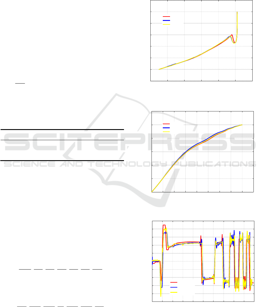
Figure 1: The altitude-velocity profiles in three methods.
Figure 2: The ground tracks in three methods.
Figure 3: The bank angle profiles in three methods.
2000 3000 4000 5000 6000 7000 8000
Velocity(m/s)
20
30
40
50
60
70
80
90
A
ltitude(km)
SCP
PSCP
hp-PSCP
10 20 30 40 50 60 70 80 90 100
Longitude(°)
-20
-10
0
10
20
30
40
Latitude(°)
SCP
PSCP
hp-PSCP
0 200 400 600 800 1000 1200 1400 1600 1800 2000
Time(s)
-100
-80
-60
-40
-20
0
20
40
60
80
100
Bank angle(°)
SCP
PSCP
hp-PSCP
Entry Trajectory Optimization via hp Pseudospectral Convex Programming
67

The solutions in three methods are shown in
Fig.1-3. The altitude-velocity profiles and ground
tracks basically coincide. The entry trajectory is very
smooth. The bank angle profiles have similar trend
with slight difference, which may result from
different discretization methods.
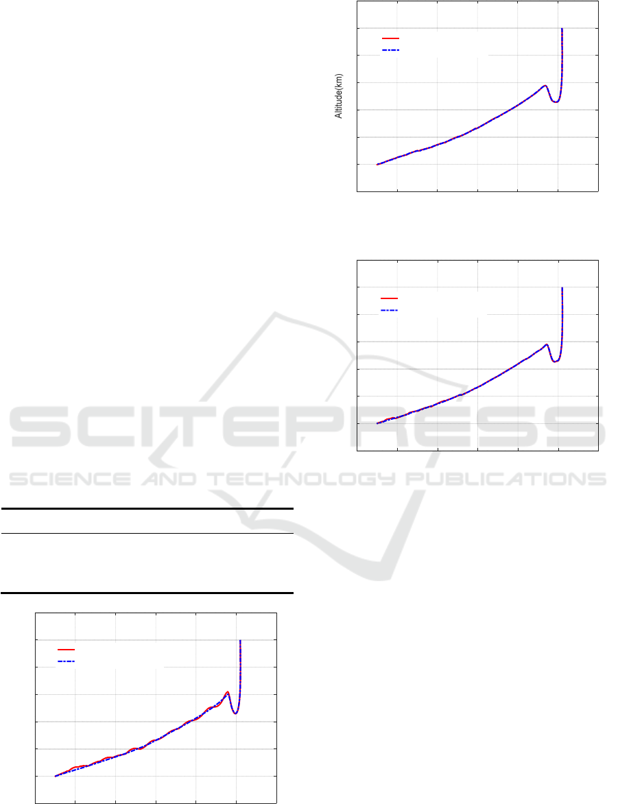
To verify the accuracy of the solutions, we
compare the optimal trajectories and trajectories
obtained by propagating the dynamics equations (1)
with optimal controls in three methods. The classical
Runge-Kutta method is used and the terminal
condition of propagation is reaching the terminal
velocity. The propagated and optimal trajectories are
displayed in Fig.4-6. The errors between the optimal
terminal states and the propagated terminal states are
given in Tab.2. As we can see, in the Fig.4-6, the
propagated trajectory does not coincide with the
optimal trajectory in SCP, while the propagated and
optimal trajectories match well in PSCP and hp-PSCP.
In Tab.2, the terminal errors of SCP, especially the
terminal longitude and latitude errors are quite large,
which is unacceptable even though the CPU time is
the shortest. As for PSCP, the terminal accuracy is
very high. However, the CPU time is one order higher
than the other two methods. By contrast, the proposed
hp-PSCP reduces the terminal errors significantly
with respect to SCP with little growth of CPU times.
In other words, the hp-PSCP method achieves a good
trade-off between computational accuracy and speed.
Table 2: Comparison of Terminal errors and CPU times for
each iteration.
States
e
h
(m)
e

(°)
e

(°)
e
V
(m/)
CPU time
SCP -61.6 1.61 0.61 -1.34 0.12
PSCP 20.3 -0.007 0.01 -1.42 2.45
Hp-PSCP 25.3 -0.04 0.05 -1.71 0.21
Figure 4: The propagated and optimal trajectories in SCP.
Figure 5: The propagated and optimal trajectories in PSCP.
Figure 6: The propagated and optimal trajectories in hp-
PSCP.
5 CONCLUSION
In this paper, the hp pseudospectral method and
sequential convex programming are combined to
solve the entry trajectory optimization problem. The
hp flipped Radau pseudospectral method is employed
to get more accurate results without much larger
computational cost compared to standard convex
approaches. Numerical results confirm that the
proposed method results in a significant decline of
computation time with limited impact on solution
accuracy with respect to pseudospectral convex
programming. Future work includes the intensive
study of the influence of h and p on solution results,
and we will apply hp-PSCP to onboard guidance.
2000 3000 4000 5000 6000 7000 8000
Velocity(m/s)
20
30
40
50
60
70
80
90
Altitude(km)
Propagated trajectory
Optimal trajectory
2000 3000 4000 5000 6000 7000 8000
Velocity(m/s)
20
30
40
50
60
70
80
90
Propagated trajectory
Optimal trajectory
2000 3000 4000 5000 6000 7000 8000
Velocity(m/s)
20
30
40
50
60
70
80
90
Altitude(km)
Propagated trajectory
Optimal trajectory
ICINCO 2019 - 16th International Conference on Informatics in Control, Automation and Robotics
68

ACKNOWLEDGMENT
This work is supported by the National Natural
Science Foundation of China (No. 11572036).
REFERENCES
Andersen, E. D., Roos, C., & Terlaky, T. (2003). On
implementing a primal-dual interior-point method for
conic quadratic optimization. Mathematical
Programming, 95(2), 249-277.
Acikmese, B., & Ploen, S. R. (2005). A powered descent
guidance algorithm for Mars pinpoint landing. In AIAA
Guidance, Navigation, and Control Conference and
Exhibit (p. 6288).
Acikmese, B., & Ploen, S. R. (2007). Convex programming
approach to powered descent guidance for mars
landing. Journal of Guidance, Control, and Dynamics,
30(5), 1353-1366.
Betts, J. T. (1998). Survey of numerical methods for
trajectory optimization. Journal of guidance, control,
and dynamics, 21(2), 193-207.
Boyd, S., & Vandenberghe, L. (2004). Convex
optimization. Cambridge university press.
Blackmore, L., Acikmese, B., & Scharf, D. P. (2010).
Minimum-landing-error powered-descent guidance for
Mars landing using convex optimization. Journal of
guidance, control, and dynamics, 33(4), 1161-1171.
Fahroo, F., & Ross, I. M. (2008, August). Advances in
pseudospectral methods for optimal control. In AIAA
guidance, navigation and control conference and
exhibit (p. 7309).
Lu, P., & Liu, X. (2013). Autonomous trajectory planning
for rendezvous and proximity operations by conic
optimization. Journal of Guidance, Control, and
Dynamics, 36(2), 375-389.
Lu, P. (2014). Entry guidance: a unified method. Journal of
Guidance, Control, and Dynamics, 37(3), 713-728.
Liu, X., Shen, Z., & Lu, P. (2015). Entry trajectory
optimization by second-order cone programming.
Journal of Guidance, Control, and Dynamics, 39(2),
227-241.
Liu, X., Shen, Z., & Lu, P. (2015). Solving the maximum-
crossrange problem via successive second-order cone
programming with a line search. Aerospace Science
and Technology, 47, 10-20.
Liu, X., Shen, Z., & Lu, P. (2016). Exact convex relaxation
for optimal flight of aerodynamically controlled
missiles. IEEE Transactions on Aerospace and
Electronic Systems, 52(4), 1881-1892.
Liu, X., & Shen, Z. (2016). Rapid smooth entry trajectory
planning for high lift/drag hypersonic glide vehicles.
Journal of Optimization Theory and Applications,
168(3), 917-943.
Lofberg, J. (2004). YALMIP: A toolbox for modeling and
optimization in MATLAB. In Proceedings of the
CACSD Conference (Vol. 3).
Patterson, M. A., & Rao, A. V. (2014). GPOPS-II: A
MATLAB software for solving multiple-phase optimal
control problems using hp-adaptive Gaussian
quadrature collocation methods and sparse nonlinear
programming. ACM Transactions on Mathematical
Software (TOMS), 41(1), 1.
Phillips, T. H. (2003). A common aero vehicle (CAV)
model, description, and employment guide. Schafer
Corporation for AFRL and AFSPC, 27.
Sagliano, M. (2017). Pseudospectral convex optimization
for powered descent and landing. Journal of Guidance,
Control, and Dynamics, 41(2), 320-334.
Sagliano, M. (2018). Generalized hp Pseudospectral
Convex Programming for Powered Descent and
Landing. In 2018 AIAA Guidance, Navigation, and
Control Conference (p. 1870).
Wright, S. J. (1997). Primal-dual interior-point methods
(Vol. 54). Siam
Wang, Z., Liu, L., & Long, T. (2017). Minimum-Time
Trajectory Planning for Multi-Unmanned-Aerial-
Vehicle Cooperation Using Sequential Convex
Programming. Journal of Guidance, Control, and
Dynamics, 40(11), 2976-2982.
Wang, Z., & Grant, M. J. (2017). Optimization of
Minimum-Time Low-Thrust Transfers Using Convex
Programming. Journal of Spacecraft and Rockets,
55(3), 586-598.
Wang, Z., & Grant, M. J. (2017). Constrained trajectory
optimization for planetary entry via sequential convex
programming. Journal of Guidance, Control, and
Dynamics, 1-13.
Wang, Z., & Grant, M. J. (2018). Autonomous entry
guidance for hypersonic vehicles by convex
optimization. Journal of Spacecraft and Rockets, 55(4),
993-1006.
Wang, J., Cui, N., & Wei, C. (2019). Optimal Rocket
Landing Guidance Using Convex Optimization and
Model Predictive Control. Journal of Guidance,
Control, and Dynamics, 1-15.
Entry Trajectory Optimization via hp Pseudospectral Convex Programming
69