A Hierarchical Planner based on Set-theoretic Models: Towards

Automating the Automation for Autonomous Systems

Bernd Kast

1 a

, Vincent Dietrich

1 b

, Sebastian Albrecht

1 c

, G. Wendelin Feiten

1 d

and Jianwei Zhang

Siemens AG, Corporate Technology, Otto-Hahn-Ring 6, 81739 Munich, Germany

University of Hamburg, Faculty of Mathematics, Informatics and Natural Sciences,

Vogt-K

olln-Str. 30, 22527 Hamburg, Germany

Keywords:

Hierarchy, Planning, Autonomy.

Abstract:

The complexity of today’s autonomous systems renders the manual engineering of control strategies or be-

haviors for all possible system states infeasible. Therefore, planning algorithms are required that match the

capabilities of the system to the tasks at hand. Solutions to typical problems with robotic systems combine

aspects of symbolic action planning with sub-symbolic motion planning and control. The problem complexity

of this combination currently prohibits online planning without task speciﬁc, manually deﬁned heuristics. To

counter that we use a set-theoretic approach to model declarative and procedural knowledge which allows for

ﬂexible hierarchies of planning tasks. The coordination of the planning tasks on different levels, the classiﬁ-

cation of information and various views on data are the core functions of hierarchical planning. We propose

suitable graph structures to capture all relevant information and discuss the elements of our hierarchical plan-

ning algorithm in this paper. Furthermore, we present two use-cases of an autonomous manufacturing system

to highlight the capabilities of our system.

1 INTRODUCTION

Setting up autonomous systems still requires huge in-

tegration and engineering efforts. In order to make

them widely applicable, we need a holistic approach

that even considers aspects of component integration.

This is especially important in production, where a

higher degree of automation, notably for small lot

sizes, can account for changing customer demands.

A limiting factor of today’s automation strate-

gies is the interwoven product and production design

which requires costly manual effort even for small

changes of some component (Hitomi, 2017), (Bryan

et al., 2007). To reduce this effort, the design process

of the product and the production system have to be

decoupled (Hu et al., 2011) and then matched again

by an autonomous system. Thus, the autonomous sys-

tem has to solve on its own certain engineering tasks

https://orcid.org/0000-0001-7838-3142

https://orcid.org/0000-0003-0568-9727

https://orcid.org/0000-0002-3647-4043

https://orcid.org/0000-0002-7593-6298

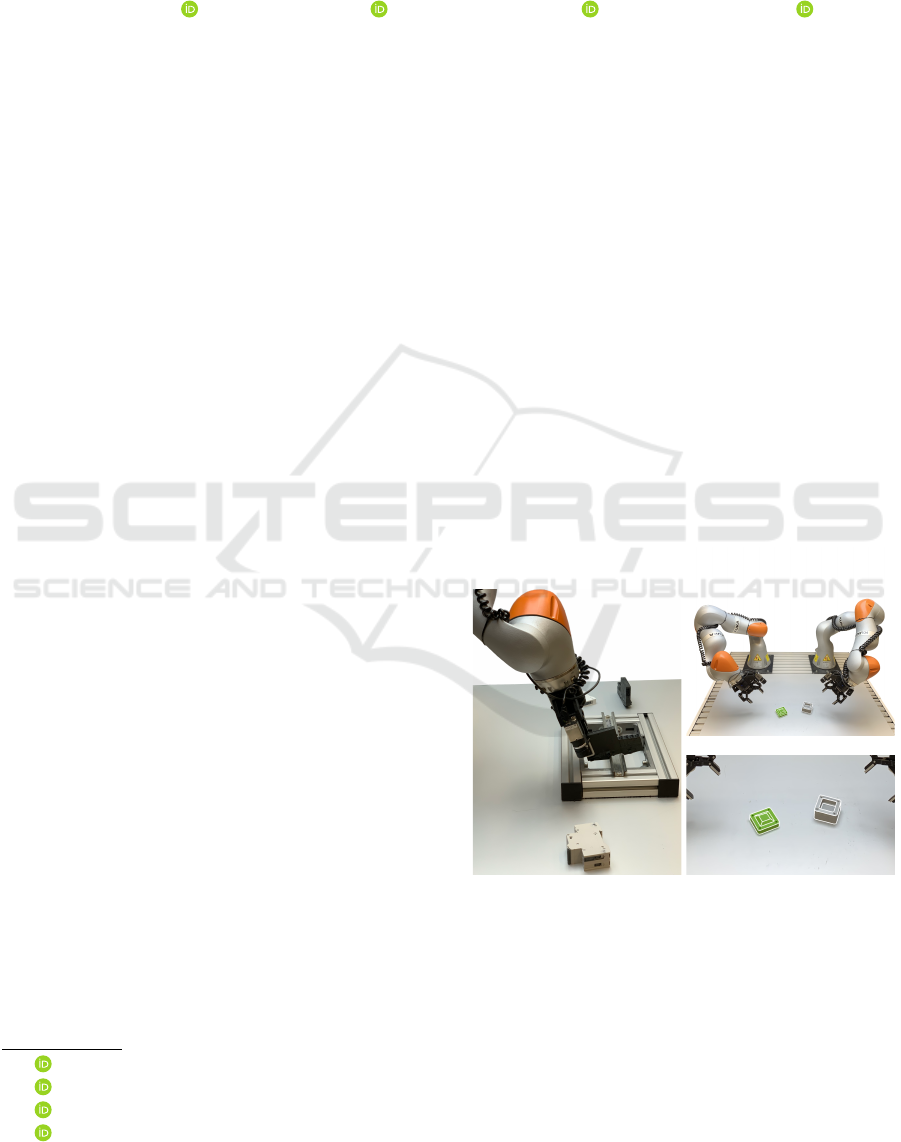
Figure 1: Images of the robotic system (upper right) and

the hat-rail with components (left) and the box next to its

lid (lower right).

that these days are addressed manually when automat-

ing a production system, i.e. the automation of au-

tomation (Schmitz et al., 2009) is necessary for ﬂexi-

ble autonomous systems.

This requires general models which character-

ize objects by their properties (declarative knowl-

edge) and describe actions modifying them (proce-

dural knowledge). These models deﬁne domains for

Kast, B., Dietrich, V., Albrecht, S., Feiten, G. and Zhang, J.

A Hierarchical Planner based on Set-theoretic Models: Towards Automating the Automation for Autonomous Systems.

DOI: 10.5220/0007840702490260

In Proceedings of the 16th International Conference on Informatics in Control, Automation and Robotics (ICINCO 2019), pages 249-260

ISBN: 978-989-758-380-3

249

suitable planners. Real-world manufacturing domains

suffer from a huge computational complexity due to

their mixed continuous and discrete nature. Dis-

crete symbolic action planning and scheduling bring

in the problem of combinatorial explosion while sub-

symbolic tasks such as motion planning or control in-

troduce time, accuracy and stability constraints. A

common approach to address this curse of dimension-

ality is to use abstractions or hierarchies to decom-

pose the problem. This allows to extract smaller sub-

problems that are easier to handle. It is especially im-

portant to deduce those hierarchies for both, proce-

dural and declarative knowledge, automatically from

the models in order to keep the task and plant descrip-

tion separate. Additionally, assumptions that limit the

ﬂexibility of the system have to be avoided. One ex-

ample is the downward reﬁnement property which de-

mands that each coarse plan can be reﬁned on all more

detailed levels. This is in general not viable for real-

world problems with decoupled models for the prob-

lem and the plant. This becomes obvious for task spe-

ciﬁc sub-symbolic properties, such as possible grasp

positions, which can for the general case not be mod-

eled on an abstract, purely symbolic level.

Throughout this paper, we illustrate our approach

with an industrial assembly use-case, cf. Figure 1,

which is modeled for maximal ﬂexibility. This means

in particular, that not only the actions of the robot,

but even the interplay between software components

is planned, cf. section 8. We present a planner that

beneﬁts from models that integrate declarative and

procedural knowledge and allow for an automatic cal-

culation of abstractions. This planner uses the graph

structures of our models on different abstraction lev-

els to factorize the problem, integrates special single-

level planners for individual subproblems but does not

depend on the downward reﬁnement property.

The paper is structured as follows: In section 2

we present related work regarding hierarchical sym-

bolic planning, combined task and motion planning in

robotics and autonomous production systems. After

that, we discuss a set-theoretic approach for declara-

tive and procedural models that natively enables the

deduction of hierarchical structures in section 3. The

data structures for the single-level planning are de-

scribed in section 4 and the respective single-level

planner is discussed in section 5. In section 6 we

extend these concepts for the hierarchical planning

context. Finally, we present the hierarchical planning

method in section 7 and demonstrate its features on

two examples in section 8.

2 RELATED WORK

Planning algorithms are often tailored to modeling

languages and rely on their expressiveness. In this

section we discuss both symbolic and sub-symbolic

planning, as well as the application speciﬁc aspects

related to for autonomous production systems.

2.1 (Hierarchical) Action Planning

The key for ﬂexible systems is a modeling language

that formalizes the description of the domain. On

the symbolic level, there are many languages such as

PDDL (McDermott et al., 1998) and its dialects that

focus on the procedural knowledge of a domain. A

long series of planning competitions have resulted in

a large set of fast planners for PDDL domains such

as (Helmert, 2006). Extensions to PDDL add sup-

port for certain sub-symbolic properties such as time.

An example is PDDL+ (Fox and Long, 2002) that

introduces events and processes to model exogenous

change and support domains with mixed discrete and

continuous dynamics. Corresponding solvers, such as

(Cashmore et al., 2016) or (Piotrowski et al., 2016),

make use of this representation and handle domains

with nonlinear continuous change. They approximate

the dynamics of the system and handle the result-

ing discretized model with uniform time steps and

step functions. Other PDDL dialects, e.g. (Dornhege

et al., 2009), extend the formalism by using seman-

tic attachments that allow for an evaluation of exter-

nally speciﬁed functions. Though, this requires mod-

ifying standard PDDL planners and to create domain-

speciﬁc PDDL action choosing the speciﬁc external

functions.

Another approach is partial-order planning (POP)

(Young et al., 1994) which involves partially spec-

iﬁed action decompositions. In this approach, the

planner is only allowed to ﬁll in missing pieces of a

ﬁxed plan template which hugely reduces the search

space. However, it is difﬁcult to ensure the separation

of hardware and task description with this approach,

which reduces the ﬂexibility.

A large community addresses hierarchical task

networks (HTN) that reﬁne each abstract skill by a

network of sub-methods, e.g. (Castillo et al., 2006),

(Goldman, 2006), (Nau et al., 2003). In their ba-

sic form they were state-oriented and could not deal

with time constraints or concurrent actions. Never-

theless, the formalism is more expressive than that of

ﬁrst principle planners (Erol et al., 1994), HTN meth-

ods can improve planning times (Nau et al., 2003)

and even support plan reparation (Gateau et al., 2013).

In (Bercher et al., 2016) an overview of HTN meth-

ICINCO 2019 - 16th International Conference on Informatics in Control, Automation and Robotics

250

ods is provided that discusses the expressiveness of

hierarchical planning formalisms as well as implica-

tions of preconditions and effects of abstract meth-

ods. A mandatory and limiting condition for HTNs

is the downward reﬁnement property that enforces re-

ﬁnements to all abstract solutions (Bacchus and Yang,

1994). Yet, the generation of suitable abstract models

for a domain is a challenging or even impossible task

and often results in a coupling between task and hard-

ware description.

This becomes obvious in (Marthi et al., 2008).

They propose expressive models, which allow for the

deﬁnition of domains with the downward reﬁnement

property. In this approach, an underlying semantic

that deﬁnes preconditions and effects even for abstract

tasks, ensures that abstract plans can always be re-

ﬁned to a primitive solution. However, this demands

that all relevant effects and preconditions of the prim-

itives have to be considered even on the most abstract

level. This is only possible if all properties can be de-

scribed symbolically and hugely limits the beneﬁts of

the hierarchical abstractions.

To overcome the limitations induced by the down-

ward reﬁnement property, several variants of HTN

planning and hybrid planning (Kambhampati et al.,

1998), (Schattenberg, 2009) have been proposed. The

hierarchical partial-order planner, introduced in (Be-

chon et al., 2014), uses additional knowledge that de-

scribes sets of abstract actions with optional methods

to increase ﬂexibility during reﬁnement. Another ap-

proach to improve versatility is the combination of

HTN and POP in a domain-speciﬁc planner with a

strict separation between several hierarchical levels

(Castillo et al., 2003). In both approaches the effects

of the downward reﬁnement property are mitigated at

the cost of models which are dependent on the hard-

ware and the task at the same time.

Temporal reasoning within an HTN planner is dis-

cussed in (Castillo et al., 2006) and an HTN ex-

tension for (nonlinear) continuous temporal environ-

ments can be found in (Molineaux et al., 2010),

in which the SHOP2 planner (Nau et al., 2003) is

matched to features from PDDL+ (Fox and Long,

2002). Those approaches offer a suitable perfor-

mance even in domains with sub-symbolic properties

but don’t support general geometric constraints such

as collisions. An overview of HTN planning can be

found in (Georgievski and Aiello, 2015).

Each of those approaches extends the application

area. Summarizing we state that manually drafted hi-

erarchies, the strict requirement of the downward re-

ﬁnement property or a limited support of continuous

properties prevents an application in our general man-

ufacturing domain.

2.2 Combined Task and Motion

Planning in Robotics

A challenging and widely discussed subproblem for

autonomous systems in production is task and mo-

tion planning. In (Srivastava et al., 2014) existing

task planners and motion planners are combined by

the introduction of new symbolic abstractions. Mo-

tion planning is used to reﬁne the plans from symbolic

planning to a sub-symbolic level. The general idea

is to add further abstract poses to the symbolic plan-

ning problem every time the reﬁnement failed because

no collision-free path could be found. This allows

to consider continuous properties on an abstract level

without manual prior modeling. However, the com-

putational complexity is shifted to the abstract level.

The advantages of the hierarchy are additionally re-

duced by the limited number of abstractions that are

possible with this approach.

Instead of combining of two separate planners

(Garrett et al., 2015) extends the symbolic planners

and their heuristics to motion planning and thus lifts

the sub-symbolic world to the symbolic planning. The

heuristic is based on domain-dependent literals that

represent reachability for example, which can be eval-

uated lazily on demand. The planner maintains a

corresponding reachability graph of sampled conﬁg-

urations. Geometric constraint-satisfaction problems

(CSP) determine plan templates with unbound vari-

ables like robot and object poses (Lozano-P

erez and

Kaelbling, 2014). The central disadvantages of these

approaches are that a discretization has to be speciﬁed

in advance and that they run into scalability issues if

a ﬁne discretization is needed.

Another possibility is to add the symbolic prop-

erties to the sub-symbolic path planning problem. If

a simple symbolic planner is used to generate action

sequences, large optimization problems can be for-

mulated that determine optimal intermediate and ﬁ-

nal states (Toussaint, 2015). They demonstrated the

strength of their approach for a stacking problem in

which towers of cylinders and plates have to be as-

sembled. However, it is computationally too demand-

ing for online planning and scales exponentially with

the number of involved objects.

The ScottyActivity planner (Fernandez-Gonzalez

et al., 2018) is one of the few approaches that con-

sider dynamics and/or temporal constraints along the

manipulation problem. It combines strong heuristics

with convex optimization and relaxed plan graphs.

However, the absence of obstacles and the limitation

to linear dynamics for the robots prohibits the appli-

cability for real-world problems.

In (Schmitt et al., 2017) an asymptotically optimal

A Hierarchical Planner based on Set-theoretic Models: Towards Automating the Automation for Autonomous Systems

251

manipulation planner is proposed that considers both,

nonlinear dynamics and collisions. Without any hier-

archical decomposition or heuristics, their approach,

which extends sampling-based roadmap planners to

explore conﬁguration spaces, scales exponentially.

2.3 Autonomous Production Systems

There are three main challenges for autonomous

robotics in production: planning to generate a coarse,

symbolic plan, mapping the plan to the actual hard-

ware and controlling it accordingly. The pioneering

system (Kaufman et al., 1996) is one of the few who

proposed an integrating approach to target all three

challenges at a time. However, this approach relied

on substantial task speciﬁc manual modeling of sub-

assemblies, which limits ﬂexibility. Additionally, the

approach is tested in simulation only and therefore it

neglects sensor input and generates a nominal control

code only. In (Thomas and Wahl, 2010) an improved

version is presented that uses CAD data and other

models to compute assembly sequences that comply

with the desired goal conﬁguration. The optimal plan

is chosen, mapped to the robot’s skills and executed

on the hardware. Due to the lack of a hierarchical de-

composition, this approach, however, suffers from the

curse of dimensionality.

3 FORMAL MODELS

The planning process requires models for declara-

tive and procedural knowledge. For our hierarchi-

cal planning approach, it is especially important that

both types are naturally hierarchically structured and

that these hierarchies match each other. We accom-

plish that with the following set-theoretic deﬁnitions,

which have been introduced in more detail in (Kast

et al., 2019).

3.1 Concepts

In this work we use the term concepts for elements of

the declarative knowledge. An example of such a con-

cept is a simple box. Each speciﬁc box is an instance

of the abstract concept ”box”, but the properties of

boxes differ in detail. For example, the shape might

be different, as one box is cubic and the other cylin-

drical. Thus, we have an abstract concept of a box and

two specializations capturing subsets. This notion of

concepts can be formally grounded by following set-

theoretic deﬁnitions:

• A concept base B

is the set of instances, not nec-

essarily ﬁnite.

• A concept C is a subset of B

, i.e., C ⊆ B

• A concept class Γ is the set of concepts C

that

have a common concept base B

, i.e.,

∀ C

∈ Γ, b ∈ C

: b ∈ B

• A partial order M , describing more detailed than,

can be deﬁned on Γ: (C

) ∈ M iff C

⊂ C

Extending the previous example: In most cases

you do not only want to know the shape of the box

but also the characteristics of the dimensions. Fur-

ther properties, like the weight or the current location,

might also be interesting. This directly leads to spe-

cial types of concepts, which we call composite con-

cepts.

The following deﬁnitions introduce composite

concepts formally:

• Given an ordered set R of identiﬁers, e.g. strings,

its elements r ∈ R are called roles. Thus, for each

subset R

⊆ R with n

:= |R

| there exists a bi-

jective mapping J to N

:= {1, . . . , n

}, i.e.,

J (r) ∈ N

∀r ∈ R

and J

−1

(n) ∈ R

∀n ∈ N

• A composite, recursively deﬁned concept C =

r∈R

with R

being the speciﬁc set of roles

for this composite concept

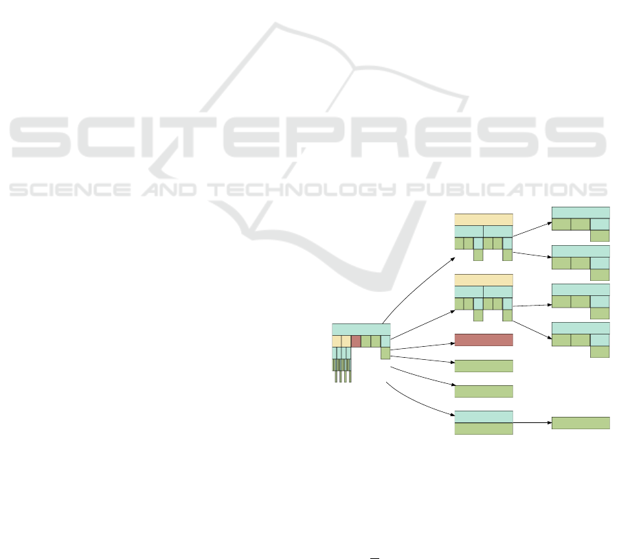
This deﬁnition of a composite concept corre-

sponds to a (directed) graph, cf. Figure 2: the nodes

correspond to (sub-)concepts and the edges point

from the composites to their sub-concepts.

std_msgs__String

SceneObject

std_msgs__Float64

Connection

std_msgs__String

AssemblyLight

std_msgs__String

AssemblyLightScrew

object_type

objects[]

length

available_connections[]

current_connections[]

object_id

Figure 2: Example of a composite concept that describes

objects in the later examples. Here, only the composite

structure of the ﬁrst level of sub-concepts is additionally de-

picted. Note that the small images for each node visualize

the composite structures. A common color is used for each

concept class. The edges are attributed with roles.

Having two composite concepts of one concept

class C,C ∈ Γ, the partial order M can be deduced

ICINCO 2019 - 16th International Conference on Informatics in Control, Automation and Robotics

252

recursively:

(C,C) ∈ M iff (C

) ∈ M ∀r ∈ R

which requires that C has all the roles of C. This

means that (see Figure 3):

∼

r∈R

∩R

× Π

r∈R

⊆ C × Π

r∈R

Γ(r)

SceneObject

AssemblyLight

sie_msgs__SceneObject

Assembly

AssemblyLightBox

AssemblyLightScrew

AssemblyScrew

AssemblyBoxLight

AssemblyScrewLight

RobotAssemblyCoarse

AssemblyBox

Figure 3: Example hierarchy of the concept class for objects

in the later examples. The graph is directed and acyclic, but

not necessarily a tree.

By deﬁnition the leaves of a concept are consid-

ered to be atomic at the modeling detail of the pro-

vided concept. Each element of a concept is called an

instance. For composite concepts this results in the

necessity to specify values for each leaf concept of a

composite concept.

In order to answer the question whether two in-

stances of the same concept represent the same thing,

we assume that for each concept C a relation, the so-

called compare relation F

, is deﬁned. This means

two instances b

, b

are similar with respect to a con-

cept C if (b

, b

) ∈ F

. The product representation al-

lows to derive similarity of two composite concepts

when all their corresponding leaves are similar. Note,

that similarity does not mean that the instances are

identical, but rather that the information provided by

the second instance does not add any additional infor-

mation on a given level of abstraction of a domain.

This compare relation will help to introduce compact

domains, in which different results are mapped to the

same graph node if the corresponding instances are

similar.

3.2 Operators

Declarative knowledge is hardly useful if elements of

the procedural knowledge, so-called operators, do not

use them. We deﬁne operators as follows (see Fig-

ure 4):

• An operator π ∈ P is a mapping of given input

concepts I

to output concepts O

with given in-

put roles r

∈ R

π,I

and output roles r

∈ R

π,O

, i.e.,

π : Π

∈R

π,I

→ Π

∈R

π,O

• The output instances can be explicitly speciﬁed by

symbolically-representable mappings (mathemat-

ical formulas) or implicitly as the result of some

calculation or experiment in simulation or the real

world, operating on input instances

• Certain operators describe modiﬁcations of in-

stances, i.e., elements of knowledge are invali-

dated when such an operator is executed; such in-

puts are called consumed. The set of roles corre-

sponding to inputs that are consumed by the oper-

ator is denoted by R

⊆ R

π,I

• Operators are fully functional, i.e., they do not

have an internal state.

AssemblyLightBox

RobotAssemblyCoarse

AssemblyLightBox

RobotAssemblyCoarse

Assemble

obj_a

obj_b

result

result_b

Figure 4: Example of an operator with multiple concepts

as in- and outputs. A consumed input is depicted by a red

edge.

Since operators are elements of a functional space,

they can also be modeled as instances of an operator

concept on a higher level of abstraction that is often

called meta level. In addition to the input and out-

put structures and a reference to the executable code,

an instance of this operator-concept can contain meta

information like key performance indicators (kpi).

A hierarchy of operators is obtained from the hi-

erarchical structures of concepts. An operator π

more detailed than another π

in case the following

conditions hold true (see Figure 7):

• all input and output roles of operator π

are ele-

ments of the role set of operator π

: R

⊂ R

and R

⊂ R

• all (common) input concepts I

r,1

and outputs

r,1

of operator π

are more detailed than those

of operator π

: (I

r,1

, I

r,2

) ∈ M ∀r ∈ R

and

r,1

, O

r,2

) ∈ M ∀r ∈ R

• the meta information, e.g. key performance indi-

cators, of operator π

are more detailed than those

of operator π

A Hierarchical Planner based on Set-theoretic Models: Towards Automating the Automation for Autonomous Systems

253

4 CONCEPTS AND GRAPHS FOR

PLANNING

In our context planning is based on the evaluation of

operators, working on the set of currently available in-

stances, to reach one or multiple goal instances. The

operators can use or consume available instances and

generate new ones. Many application domains pose

problems combining symbolic and sub-symbolic in-

stances. However, standard approaches run into the

curse of dimensionality. The approach of hierarchi-

cal planning is based on the hierarchies of concepts

and operators. It tries to solve the planning task on an

abstract level and to reﬁne the plan step by step and

abstraction level by abstraction level until a plan on

the most detailed level is obtained.

To formalize the structures obtained during plan-

ning we ﬁrst introduce formal models for a planning

task, a planner and a plan.

4.1 Planning Task

A planning task PT (X

init

, X

goal

, X

) speciﬁes the com-

bination of three sets: the set of initial instances

init

:= {b

, i = 1, . . . , n

init

}, the set of goal instances

goal

= {b

, j = 1, . . . , n

goal

} and the set of available

operators X

:= {π

, k = 1, . . . ,n

} with n

init

∈ N

and n

goal

, n

∈ N. Consequently, a planning task is a

concept in the meta domain.

4.2 Plan Family

We introduce the concept (in the meta domain) of a

plan family that contains the following information:

the initial instances, the executed operators, the input

instances of executed operators with their roles, and

the output instances of executed operators.

To represent this plan family, we use an anno-

tated bi-partite graph G

(V, E, E

con

), in which all an-

notated edges in E

con

⊆ E correspond to consumed

operator inputs. The one node set V

only contains

nodes representing instances and the other V

consists

of operators only. The bi-partite property ensures that

V = V

∪V

, V

∩V

0 and ∀e ∈ E : e = (v

, v

) with

, v

} 6⊆ V

and {v

, v

} 6⊆ V

. The representation

mapping f

: V → B ∪ P of nodes in G

to instances

and operators is assumed to be bijective.

Adding an Executed Operator to a Plan Family.

For every operator that is executed during planning,

all new nodes are added to the graph as long as the

graph does not already contain the information. The

result is the bi-partite graph (

V , E, E

con

) with V ⊆ V

and E ⊆ E. In more detail, this means that, with the

given operator π : Π

∈R

π,I

→ Π

∈R

π,O

, the ex-

ecution results in the following mapping between in-

stances:

| r ∈ R

π,I

} 7→ {b

| r ∈ R

π,O

The graph is only modiﬁed if the entropy (number of

different results for a given input set) of the operator,

is not yet exhausted by former executions. Thus, a

node v

is added to V

and all inputs are connected via

a directed edge to this new node. Edges correspond-

ing to consumed inputs are marked by adding them

to E

con

. Additionally, nodes for all output instances,

i.e., {v

−1

)

| r ∈ R

π,O

}, are added to V

and v

connected to all these outputs via directed edges.

We introduce a so-called compact domain, in

which new nodes are only added for instances that

carry new information, i.e., node v ∈ V is added

if ∀v

∈ V

with v

6= v : ( f

), f

(v)) 6∈ M or

( f

(v), f

)) 6∈ M . If the plan family already con-

tains a node related to an instance with the same infor-

mation as the output instance, the mapping f

points

to that node instead. Thus, compact domains have a

considerably smaller number of nodes enabling better

scaling. In particular, the number of considered oper-

ators during planning can exceed the number of nodes

in the corresponding plan family (see Table 1 for the

graph sizes in the robotic example). Note that in con-

sequence a plan family in a compact domain can have

cycles, since the operator outputs can be mapped to

ancestor nodes of the operator node v

Thus, the following equations hold for the sets of

the plan family:

= V

∪ {v

= V

∪

−1

)



r ∈ R

π,O

E = E ∪

n

−1

)

, v





r ∈ R

π,I

∪

n

, v

−1

)





r ∈ R

π,O

con

= E

con

∪

n

−1

)

, v





r ∈ R

π,I

4.3 Planner State Graph

Planning considers sets of instances X

, i ∈ N. The

initial set is X

init

. A plan is available if, by applying

operators, a set X

is generated that fulﬁlls the goal

set X

goal

, i.e.,

∀b

∈ X

goal

∃b

∈ X

: (b

, b

) ∈ F

in which b

∈ C

. Each set of instances X

is obtained

by executing one operator π

∈ X

, k ∈ N, on one

selection of instances (b

, . . . , b

) with n

:= |R

ICINCO 2019 - 16th International Conference on Informatics in Control, Automation and Robotics

254

from a previous set of instances X

, j ∈ {0, . . . , j − 1}

(with X

:= X

init

= (X

∪ π

, . . . , b

)) \ {b

ˆn

| J

−1

( ˆn) ∈ R

in which the instances have to be an element of the

correct concept type b

J (r

)

∈ C

∩ X

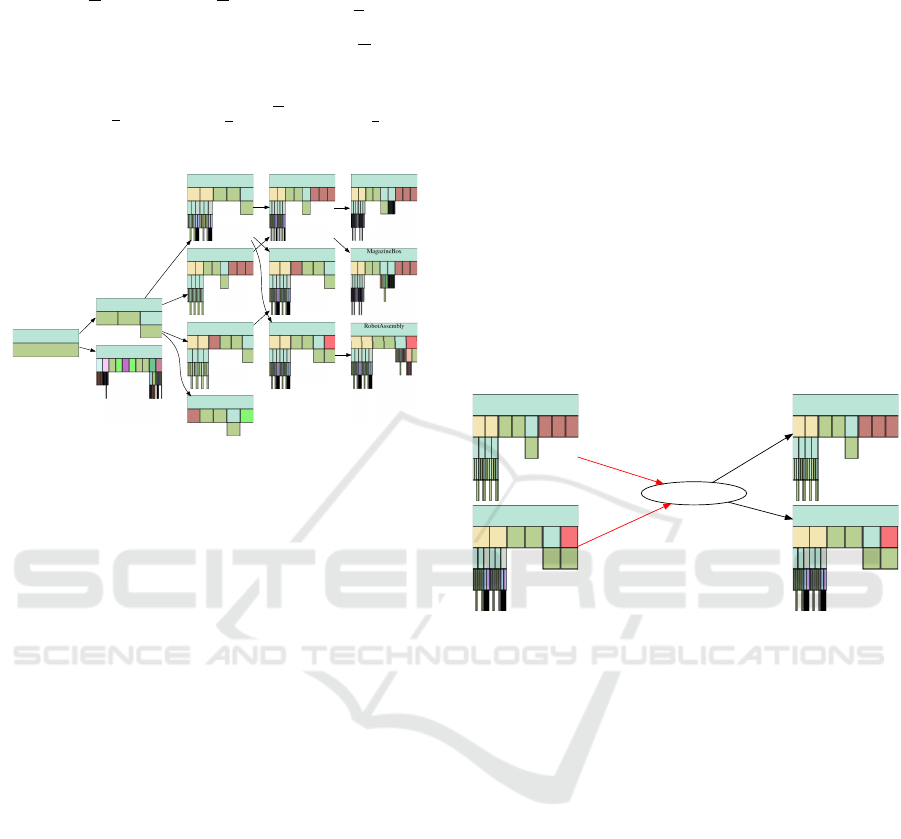
Figure 5: Part of the planner state graph for the later exam-

ple of a hat-rail assembly.

Therefore, we introduce a directed graph

(V, E) to describe the planner state as shown in

Figure 5. Each node v

∈ V corresponds to a set of

instances X

(and a subgraph of the plan family).

There exists a directed edge e = (v

, v

) ∈ E iff X

was

obtained from X

by applying an operator. We assume

a compact graph structure similar to a compact

domain, i.e., ∀v

, v

∈ V, v

6= v

: X

\ X

∪ X

\ X

This property reduces the size of the planning space

considerably, because plan duplication is avoided for

similar paths leading to the same intermediate planner

state X

. Additionally, this structure allows to detect

dead ends, which is later used by the backtracking

techniques for hierarchical planning.

5 SINGLE-LEVEL PLANNING

The classical planning problem is named single-

level planning (SLP) as it doesn’t consider hierar-

chies of concepts or operators. A planning task

PT (X

init

, X

goal

, X

) is solved in a constructive manner

by applying operators from X

to available instances.

A planning step is comprised by three actions:

1. choose the planning node v

with the correspond-

ing instances X

to proceed from,

2. select an operator π

∈ X

with its input concepts

for r ∈ R

3. single out instances from X

and map them to the

inputs of π

such that b

∈ I

∀r ∈ R

This general structure is valid for all kinds of

planners ranging from PDDL to motion planning.

Even classical graph algorithms like depth-ﬁrst and

breadth-ﬁrst search can be used to realize such a

single-level planner. In our implementation we let

the search algorithm determine the next node v

and

iterate over all operators and all possible combina-

tions of corresponding input instances for that state.

More evolved planners have either better heuristics

and sampling strategies or use suitable problem re-

formulations for speciﬁc sub-problems. Nevertheless,

the core elements of forward planners correspond to

the three steps described above.

Since each node v

corresponds both to a set of

instances X

and a subgraph of the plan family, this

subgraph captures the respective plan if the goal in-

stances X

goal

are met by the instances of X

6 GRAPHS FOR HIERARCHICAL

PLANNING

The computational complexity of the planning prob-

lem, which results from the mixture of symbolic and

sub-symbolic properties, can be handled if hierarchies

of suitable concepts and operators are considered.

The core idea is to generate a plan on an abstract

level where only a few instances and operators exist.

Then each step of this plan has to be recursively re-

ﬁned until the maximal level of detail is reached for

all operators. In case a plan step cannot be reﬁned on

a more-detailed level, a back-tracking procedure is re-

quired that is described in subsection 7.2. This hierar-

chical divide and conquer approach ideally scales log-

arithmically with the number of required plan steps.

Nevertheless, it is only beneﬁcial with the right num-

ber of layers, if abstract plans sort out steps that are

less promising on a more detailed level and if the

downward reﬁnement property holds often, thus most

steps can be reﬁned later on. In turn this requires the

models of the concepts and operators to be suitably

structured. Determining such models is a hard task

on its own. However, the set-theoretic approach of the

introduced formal models for concepts and operators

helps to manually or automatically deﬁne them.

6.1 Parent Child Mapping

A central aspect of hierarchical planning is to reﬁne

an operator by posing a new planning task on a more-

detailed level. This mainly corresponds to a selec-

A Hierarchical Planner based on Set-theoretic Models: Towards Automating the Automation for Autonomous Systems

255

tion of suitable operators. Thus, we introduce the set-

valued parent child mapping F

: P ⇒ P such that

(π

) := F

({π

}) = X

Currently, we assume that such a mapping is pro-

vided and engineered during modeling of operators.

For some domains an algorithmic extraction of that

mapping just from the sets of concepts and operators

was successfully tested. For general domains, how-

ever, this is a problem to be addressed in future re-

search.

In the following we introduce two graphs for a

formal description of dependencies between plans on

different levels of abstraction: the layer graph G

addresses the hierarchical dependencies between plan

steps and planning tasks, and the extended planner

state graph G

EPS

represents temporal dependencies.

These two combined with the previously described

plan family, which captures the causal dependencies

between instances and operators, could be represented

in a single multi-layer graph. In this paper we stick to

a presentation with separate graphs though as it is eas-

ier to understand.

6.2 Layer Graph

Since our planning approach does not assume a ﬁxed

number of hierarchy levels, each planning task PT de-

ﬁnes some layer. Note that consequently the number

of layers can vary during the planning process.

We introduce the (directed) bi-partite layer graph

(V, E) to capture dependencies between planning

states and layers, cf. Figure 6. Each node within the

ﬁrst set V

corresponds to a planning task. As de-

scribed in subsection 4.3, several planner states re-

sult during (single-level) planning for a given plan-

ning task. Each of these states is represented in the

layer graph by a node in the set V

. Note that the two

sets V

and V

are disjoint.

Figure 6: Part of the layer graph for the box-lid-example

(subsection 8.2). The node colors match the temporal order

during planning, compare Figure 8.

The set of vertices E represents dependencies of

two kinds, which are discriminated by the direction

relative to layer nodes. The ﬁrst type connects plan-

ner state nodes obtained during planning with their re-

spective layer nodes which represent planning tasks,

i.e., ∀e = (v

, v

) ∈ E, v

∈ V

: v

∈ V

. The second

type connects a planner state to exactly one layer node

if the layer node speciﬁes the planning task to reﬁne

the operator that led to the planner state (cf. subsec-

tion 4.3), i.e., ∀e = (v

, v

) ∈ E, v

∈ V

: v

∈ V

and

∀v

∈ V

: |{e | e = (v

, v

) ∈ E}| ≤ 1.

Consequently, the layer graph G

is tree-

structured and captures the hierarchical reﬁnements

of plans. For later references, the mapping of each

planning state to its corresponding layer is given by:

PS, L

: V

→ V

with F

PS, L

(p) := l such that (l, p) ∈ E.

6.3 Blacklist

The planning task that reﬁnes a plan step, has a re-

duced set of instances for two reasons. First, the com-

putational complexity is reduced, as less combina-

tions are possible with fewer instances. Second, this

assures that the plan is in accordance with the higher-

level plan. This is particularly important for domains

that are persistent and thus can’t be set to an arbitrary

state (e.g. real-world execution).

For example, assume that one out of two boxes

has to be moved to a different working surface. In the

coarse plan the smaller box is picked and then trans-

ported. If this pick is reﬁned, only the smaller box is

available. Otherwise, the more detailed planner could

choose the bigger box for this task and an inconsis-

tency between the plans on the different levels of ab-

straction would result.

The idea is to set all instances on a black list X

Black

that belong to a concept corresponding to an operator

input on the more abstract level. Let the coarse plan-

ning task PT(X

init

, X

goal

, X

) and a corresponding plan

be given as a plan family (V, E, E

con

∀v

∈ V

, v

∈ V

, (v

, v

) ∈ E : v

∈ X

Black

and

∀v

∈ V

, v

∈ X

Black

, v

∈ C : v

∈ X

Black

Let v

∈ V

be one operator in the plan that has no

preceding operators, i.e., ∀v

∈ V

with (v

, v

) ∈ E

holds v

∈ X

init

, then the corresponding planning task

for reﬁnement is:

( X

init

\ X

Black

∪ {v

| (v

, v

) ∈ E},

| (v

, v

) ∈ E},

(π

)).

If the operator has predecessors, the set of initial

instances has to be replaced by resulting instances of

the reﬁnement of that preceding operator. In order

to formally capture these dependencies, we have to

extend the planner state graph G

of the single-level

planning.

ICINCO 2019 - 16th International Conference on Informatics in Control, Automation and Robotics

256

6.4 Extended Planner State Graph

Hierarchical planning requires encoding of temporal

relations between instances of different layers. There-

fore, we extend the planner state graph G

and dis-

cuss the related blacklists.

A single-level plan that resulted from a reﬁnement

step, is deﬁned by the sequence of planning states in

the G

and a blacklist X

Black

. The planning task corre-

sponds to the ﬁrst planning state p

in that sequence

as it maps to the layer node in the layer graph. Solv-

ing this task results again in a separate planner state

graph. However, the goal is to combine all planner

state graphs in one large graph, the extended planner

state graph G

EPS

, for uniﬁed data handling during hier-

archical planning. Thus, we extend the node informa-

tion of the (one-layer) planner state graphs by their

layer information given by F

PS, L

to avoid mixing of

layers.

Assuming that a reﬁning plan for the planner state

is found, the deﬁnition of the planning task corre-

sponding to the layer l

i+1

= F

PS, L

i+1

) has to use

the resulting instances of that plan. Therefore, we

add one additional node to G

EPS

(V, E) for each plan-

ner state that reached the goal set X

goal

. Let p

such a planning state and v be the corresponding addi-

tional node, then a matching edge is added (p

, v) ∈ E.

The set of instances corresponding to the node v con-

tains the union of instances from the preceding node

X(p

) and the blacklisted instances in the correspond-

ing layer X

Black

(l): X(v) := X(p

) ∪ X

Black

(l).

In order to reﬁne the next planner state of the

coarse plan, one of the plans reﬁning the preceding

node has to be selected, leading to the node with

blacklisted instances v. Let the planner state p

i+1

cor-

respond to the operator π in the plan family G

. Now,

the set of blacklisted instances for the next layer can

be speciﬁed:

Black

i+1

) := (X(v) ∩ X

Black

)

\{v

| (v

, π) ∈ E

, (v

, v

) ∈ F}.

Then the set of initial instances for the next layer l

i+1

results: X

init

i+1

) := X(v)\ X

Black

i+1

This means that for each plan reﬁning the previ-

ous planner state p

a new set of initial instances re-

sults and a corresponding new layer is generated. To

also keep track of these dependencies, we add fur-

ther edges to the extended planner state G

EPS

linking

the node v with the added blacklist elements to the

planner state p corresponding to the initial instances

init

i+1

7 HIERARCHICAL PLANNING

The goal of hierarchical planning is to ﬁnd a sequence

of planner states in G

EPS

such that no corresponding

operator has a further reﬁnement. For this task, the

graphs of the plan family G

, the extended planner

state G

EPS

and the layers G

are used.

The basic idea to reduce the fanout and thus

counter the curse of dimensionality, is to use prior

knowledge that is encoded by abstractions, like visu-

alized in Figure 7. Once a plan was found on an ab-

stract level, each step in this plan deﬁnes a new plan-

ning task that can either be reﬁned by a single, more

detailed operator or poses a new planning task on its

own.

However, there is freedom in choosing the order

of reﬁning planning states on different levels of ab-

straction. The performance of such a reﬁnement strat-

egy depends highly on the domain at hand. If, for in-

stance, the downward reﬁnement property holds, one

can always reﬁne all operators to the most detailed

level before proceeding to the next step. On the other

hand, if some reﬁnements repeatedly fail even on a

rather coarse level, it is suboptimal to reﬁne the ﬁrst

steps to maximal detail before checking the reﬁne-

ments of later steps on coarser levels.

If a reﬁnement fails previous planning steps need

to be adapted accordingly. Such backtracking meth-

ods are the key to real-world scenarios in which the

coarser level cannot consider all details.

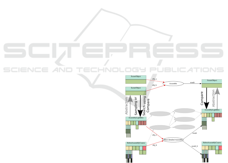
Assemble

obj_a

obj_b

result

More detailed Assemble

obj_b

obj_a

result

result_b

Figure 7: Visualization of the basic planning idea to reduce

the fanout. An abstracted planning task is obtained based on

the original instances and goals (arrows pointing upwards).

New tasks in the reﬁned level are posed by each step in the

coarse plan. Either a primitive, single operator plan exists

(white ellipse) or a planner has to be used to ﬁnd a suitable

plan (gray ellipses). The compare function is used to ensure

that the abstractions of available instances and goals comply

with the instances of the course plan.

A Hierarchical Planner based on Set-theoretic Models: Towards Automating the Automation for Autonomous Systems

257

7.1 Hierarchical Strategies

The two most basic strategies follow the spirit of

depth- and breadth-ﬁrst search and deﬁne the ex-

trema of possible approaches. Naturally, interme-

diate strategies, possibly including heuristics, could

increase planning performance for speciﬁc domains,

however this is a topic for further research.

The breadth-ﬁrst strategy reﬁnes all operators of

one level once.

7.2 Backtracking

Only the downward reﬁnement property could assure

that all plan steps can be reﬁned until the ﬁnest level is

reached. However, this property cannot be guaranteed

for all real-world problems. Therefore, the hierarchi-

cal strategies have to be complemented by backtrack-

ing procedures.

Such a backtracking method triggers re-planning

on former layers. Since the overall problem is as-

sumed to be solvable, there exists a set of layers and

some selection of corresponding plans such that all

operators are fully reﬁned.

In most cases it is reasonable to choose the back-

tracking procedure that inverts the hierarchical (for-

ward) search strategy. In the case of a breath-ﬁrst

search, tasks that are predecessors within the ex-

tended planner state G

EPS

of the failing step are con-

sidered ﬁrst. Only, if there exist no alternative plans

in these layers that lead to a succeeding reﬁnement,

the more abstract layer, i.e., an ancestor in G

of the

node given by F

PS, L

, is addressed.

Re-planning means that the original goals are

blacklisted and the (single-level) planner continues its

search then.

8 EXAMPLE: AUTONOMOUS

ASSEMBLY CELL

Our example setup consists of two robot arms with

seven degrees of freedom each, cf. Figure 1. The

workspaces of the arms have considerable overlap

to enable cooperation and wrist-mounted cameras to

perceive the environment. To demonstrate the capa-

bilities of our approach, two different use-cases are

analyzed. The ﬁrst one considers a setup for the as-

sembly of control cabinets: circuit breakers and other

components have to be automatically assembled on a

hat-rail. The focus of this example is the scalability

with an increasing number of necessary steps. The

second use-case is simpler, thus we can discuss the

backtracking algorithm on the real graph structures.

The difﬁculty for both scenarios is the combina-

tion of high dimensional continuous properties (14

degrees of freedom for the robotic arms and up to

ﬁve times three dimensions for the objects) and a

even higher number of discrete options. Those dis-

crete options not only result from the actions directly

visible on the robot, such as perception, grasping,

clicking, pushing or releasing, but also from differ-

ent sequences of varying operators that calculate pa-

rameterizations such as grasp conﬁgurations, view

poses or initialize the hardware. The operators in

our models are kept rather atomic, to ensure ﬂexibil-

ity, easy extension and composability as demanded

for autonomous manufacturing systems. Addition-

ally, these requirements result in subsection 4.3 in the

deﬁnition of planner states being the combinations of

available instances. In consequence, inhomogeneous

planner states have to be considered during planning

in opposition to most motion planner that assume a

homogeneous state for performance reasons.

8.1 Hat-rail Assembly

For the hat-rail example four components and the hat-

rail are initially placed in the working area of the

robot arm. The precise conﬁguration of the parts is

not known in the beginning, thus a perception step is

required. The goal of the task is speciﬁed on an ab-

stract level, which only states the ﬁnal position of the

components on the rail.

To actually control the robotic system the se-

quence of the four assembly operations of the coars-

est plan have to be reﬁned three times. The ﬁrst re-

ﬁnement adds further symbolic properties to the ﬁrst

domain. Then, the second reﬁnement actually simu-

lates all necessary robot motions assuring collision-

free paths and reachability. Finally, the actual control

of the robotic hardware is the most-detailed layer.

In this experimental setup we use the breadth-ﬁrst

strategy to hierarchically reﬁne the coarse plan. Our

numerical result (cf. Table 1) shows that the hierar-

chical approach scales almost linearly in the number

of pieces to be assembled, which is the best we can

expect without (automatically generated) additional

abstraction levels for longer tasks. Note, that those

planning times include all execution times of called

operations. This includes computation and simula-

tion of controllers for both robot arms considering the

full nonlinear robot dynamics (∼ 0.3 [s] per motion

task). A considerable offset for the planning times is

caused by the loading and construction of the geomet-

ric scene (∼ 1.2 [s] once). For comparison we used a

simple breadth ﬁrst search on the same problem. For

a single piece that is assembled, this algorithm is one

ICINCO 2019 - 16th International Conference on Informatics in Control, Automation and Robotics

258

order of magnitude slower than our hierarchical ap-

proach. For two pieces it took at least three orders of

magnitude longer than the hierarchical algorithm and

did not ﬁnd any solution before we ran out of mem-

ory. Arguably a faster algorithm can be found to solve

this problem, which will be faster at least for the sin-

gle piece assembly. However, the interesting point is

how the solution will scale with increasing numbers

of pieces. One can expect, that non hierarchical ap-

proaches run into the curse of dimensionality.

Table 1: Planning times t, and number of nodes in the plan

family and planner state over the number of pieces to as-

semble. The ﬁrst block states the results of the hierarchical

planner and the second block a single-level approach which

highlights the complexity of the task.

1 pc. 2 pcs. 3 pcs. 4 pcs.

t [s] 3.7 5.5 7.9 10.5

EPS

| 159 330 502 688

| 89 200 314 439

t [s] 79.2 > 7 · 10

* *

EPS

| 32,203 > 2 · 10

* *

| 981 > 4 · 10

* *

|Plan| 16 36 56 76

These results demonstrate that the hierarchy suc-

cessfully handles the curse of dimensionality. Note

that the models for this example fulﬁll the downward

reﬁnement property, thus no backtracking is needed,

which explains the almost perfect results.

8.2 Box Lid Assembly

In order to show the backtracking features of our plan-

ning approach, we consider a simple assembly pro-

cess, in which a lid has to be placed on top of a box.

The coarse level has to choose which robot arm

should pick the lid and assemble it on the box. How-

ever, the box is only reachable by one of the arms, as

it is placed outside of the workspace overlap of the

two robots. If the coarse level now chooses the wrong

arm to do this task, there exists no valid reﬁnement

on the sub-symbolic level. Therefore, backtracking is

needed. Note that only the second step of the coarse

plan cannot be reﬁned, since both arms can pick the

lid, but only one can put it on the box.

Consequently, the backtracking procedure tries to

ﬁnd an alternative plan in the temporal preceding step

ﬁrst and then chooses a new plan on the coarser layer.

See Figure 8 for a visualization of the planner state of

this example.

The orange area shows the part where no plan that

reﬁnes the second step in the coarse plan is found.

The backtracking approach then tries to ﬁnd an alter-

Figure 8: The planner state G

with backtracking. No re-

ﬁned plan is found (orange area), therefore backtracking

considers the preceding layer (red area) ﬁrst. A second plan

on the coarser level (dark green area) can then be success-

fully reﬁned (green and petrol area).

native plan in the preceding layer (red area). How-

ever, there exists no plan to pick the lid in a way that

allows assembly, with the left arm, as the box is out

of reach. Thus, the backtracking goes to the more ab-

stract level (dark green area) and selects an alternative

plan that uses the right arm instead of the left one.

Here, the backtracking stops, and the breadth-ﬁrst

search is restarted. In this second coarse plan both

actions, i.e., picking and assembling, can be reﬁned

successfully (green and petrol area, respectively).

9 CONCLUSIONS

The approach to ground the declarative and procedu-

ral knowledge on set theory enables to ﬂexibly reason

about hierarchies. Based on these structures we intro-

duce a hierarchical planner that allows to seamlessly

traverse different abstraction levels and obliterate the

differences between symbolic and sub-symbolic do-

mains. This approach additionally allows for mod-

eling robot and task description independently. This

leads to highly ﬂexible and composable systems. We

discussed examples of autonomous production sys-

tems with real hardware that is controlled with this

hierarchical approach. Our examples show that hier-

archy can help to avoid the curse of dimensionality

and backtracking allows to handle cases that do not

have the downward reﬁnement property.

REFERENCES

Bacchus, F. and Yang, Q. (1994). Downward reﬁnement

and the efﬁciency of hierarchical problem solving. Ar-

The presented research is ﬁnanced by the TransFit

project which is funded by the German Federal Ministry of

Economics and Technology (BMWi), grant no. 50RA1701,

50RA1702, and 50RA1703.

A Hierarchical Planner based on Set-theoretic Models: Towards Automating the Automation for Autonomous Systems

259

tiﬁcial Intelligence, 71(1):43–100.

Bechon, P., Barbier, M., Infantes, G., Lesire, C., and Vidal,

V. (2014). Hipop: Hierarchical partial-order planning.

In STAIRS, pages 51–60.

Bercher, P., H

oller, D., Behnke, G., and Biundo, S. (2016).

More than a name? on implications of preconditions

and effects of compound htn planning tasks. In ECAI,

pages 225–233.

Bryan, A., Ko, J., Hu, S., and Koren, Y. (2007). Co-

evolution of product families and assembly systems.

CIRP Annals, 56(1):41–44.

Cashmore, M., Fox, M., Long, D., and Magazzeni, D.

(2016). A compilation of the full PDDL+ language

into SMT. In AAAI Workshop: Planning for Hybrid

Systems.

Castillo, L., Fern

andez-Olivares, J., Garcia-Perez, O., and

Palao, F. (2006). Efﬁciently handling temporal knowl-

edge in an htn planner. In ICAPS, pages 63–72.

Castillo, L., Fern

andez-Olivares, J., and Gonzalez, A.

(2003). Integrating hierarchical and conditional plan-

ning techniques into a software design process for au-

tomated manufacturing. In ICAPS.

Dornhege, C., Eyerich, P., Keller, T., Tr

ug, S., Brenner,

M., and Nebel, B. (2009). Semantic attachments for

domain-independent planning systems. In Conf. on

Automated Planning and Scheduling.

Erol, K., Hendler, J., and Nau, D. (1994). Htn planning:

Complexity and expressivity. In AAAI, volume 94,

pages 1123–1128.

Fernandez-Gonzalez, E., Williams, B., and Karpas, E.

(2018). Scottyactivity: Mixed discrete-continuous

planning with convex optimization. Artiﬁcial Intel-

ligence Research, 62:579–664.

Fox, M. and Long, D. (2002). Pddl+: Modeling continuous

time dependent effects. In Int. NASA Workshop on

Planning and Scheduling for Space, volume 4.

Garrett, C., Lozano-P

erez, T., and Kaelbling, L. (2015).

Ffrob: An efﬁcient heuristic for task and motion plan-

ning. In Algorithmic Foundations of Robotics XI,

pages 179–195. Springer.

Gateau, T., Lesire, C., and Barbier, M. (2013). Hidden:

Cooperative plan execution and repair for heteroge-

neous robots in dynamic environments. In IROS,

pages 4790–4795. IEEE.

Georgievski, I. and Aiello, M. (2015). Htn planning:

Overview, comparison, and beyond. Artiﬁcial Intel-

ligence, 222:124–156.

Goldman, R. (2006). Durative planning in htns. In ICAPS,

pages 382–385.

Helmert, M. (2006). The fast downward planning system.

Artiﬁcial Intelligence Research, 26:191–246.

Hitomi, K. (2017). Manufacturing Systems Engineering:

A Uniﬁed Approach to Manufacturing Technology,

Production Management and Industrial Economics.

Routledge.

Hu, S., Ko, J., Weyand, L., ElMaraghy, H., Lien, T., Koren,

Y., Bley, H., Chryssolouris, G., Nasr, N., and Shpi-

talni, M. (2011). Assembly system design and oper-

ations for product variety. CIRP Annals, 60(2):715–

733.

Kambhampati, S., Mali, A., and Srivastava, B. (1998). Hy-

brid planning for partially hierarchical domains. In

AAAI/IAAI, pages 882–888.

Kast, B., Albrecht, S., Feiten, W., and Zhang, J. (2019).

Bridging the gap between semantics and control for

industry 4.0 and autonomous production. In CASE.

IEEE.

Kaufman, S., Wilson, R., Jones, R., Calton, T., and Ames,

A. (1996). The archimedes 2 mechanical assembly

planning system. In ICRA, volume 4, pages 3361–

3368. IEEE.

Lozano-P

erez, T. and Kaelbling, L. (2014). A constraint-

based method for solving sequential manipulation

planning problems. In IROS, pages 3684–3691. IEEE.

Marthi, B., Russell, S., and Wolfe, J. (2008). Angelic hier-

archical planning: Optimal and online algorithms. In

ICAPS, pages 222–231.

McDermott, D., Ghallab, M., Howe, A., Knoblock, C.,

Ram, A., Veloso, M., Weld, D., and Wilkins, D.

(1998). Pddl - the planning domain deﬁnition lan-

guage. The AIPS-98 Planning Competition Comitee.

Molineaux, M., Klenk, M., and Aha, D. (2010). Planning in

dynamic environments: extending htns with nonlinear

continuous effects. In Conf. on Artiﬁcial Intelligence,

pages 1115–1120. AAAI Press.

Nau, D., Au, T.-C., Ilghami, O., Kuter, U., Murdock, J., Wu,

D., and Yaman, F. (2003). Shop2: An htn planning

system. Artiﬁcial Intelligence Research, 20:379–404.

Piotrowski, W., Fox, M., Long, D., Magazzeni, D., and

Mercorio, F. (2016). Heuristic planning for hybrid

systems. In Conf. on Artiﬁcial Intelligence, pages

4254–4255. AAAI Press.

Schattenberg, B. (2009). Hybrid planning and scheduling.

PhD thesis, University of Ulm, Germany.

Schmitt, P., Neubauer, W., Feiten, W., Wurm, K.,

v. Wichert, G., and Burgard, W. (2017). Optimal,

sampling-based manipulation planning. In ICRA,

pages 3426–3432. IEEE.

Schmitz, S., Schluetter, M., and Epple, U. (2009). Au-

tomation of automation — deﬁnition, components and

challenges. In Conf. on Emerging Technologies &

Factory Automation. IEEE.

Srivastava, S., Fang, E., Riano, L., Chitnis, R., Russell, S.,

and Abbeel, P. (2014). Combined task and motion

planning through an extensible planner-independent

interface layer. In ICRA, pages 639–646. IEEE.

Thomas, U. and Wahl, F. (2010). Assembly planning and

task planning—two prerequisites for automated robot

programming. In Robotic Systems for Handling and

Assembly, pages 333–354. Springer.

Toussaint, M. (2015). Logic-geometric programming: An

optimization-based approach to combined task and

motion planning. In IJCAI, pages 1930–1936.

Young, R. M., Pollack, M., and Moore, J. (1994). Decom-

position and causality in partial-order planning. In

AIPS, pages 188–194.

ICINCO 2019 - 16th International Conference on Informatics in Control, Automation and Robotics

260