
Investigation of Characteristics in Mountain Area with the Aim of
Collecting Data for Modelling Flow Turbulent Parameters in a Wind
Farm Located in a Coastal Area
Sergei Strijhak
a
, Konstantin Koshelev
b
and Arina Kryuchkova
c
Ivannikov Institute for System Programming of the RAS, 25 Alexander Solzhenitsyn Street, 109004, Moscow, Russia
Keywords: Wind Energy, Wind Farm, Crete, Russia, Complex Terrain, Mountain, Large-Eddy Simulation, Finite
Volume Method, Mesh, SOWFA Library, Solver, Wind Turbines, Velocity, Pressure, Temperature, Computer
Nodes.
Abstract: The article summarize results of the study of wind farms located on the island of Crete and in Russia using
different solvers of open source SOWFA library. Applying large-eddy simulation approach allows to take
into account the orography of the area, different physical processes like lower-level jets and will assess the
impact of the wind farm and turbulent wakes on the local microclimate of the region.
1 INTRODUCTION
Wind energy is an important part of renewable energy
sources in many countries. In the last decades the
flow simulation for wind farms and turbines have
been studied more because it is a very good
alternative for producing energy. The turbulent wakes
dynamics and wind turbines performance in wind
farms are the questions of the great interest now for
the scientific community. Large-eddy simulation
(LES) has recently been well applied in the context of
numerical simulation of a flow over wind turbines on
flat and complex terrains (Mehta et al., 2014; Stevens
and Meneveau, 2017). The region of the island of
Crete encourages siting of wind farms due to the
strong wind potential and insular rough terrain
(Tsoutsos et al., 2015; Kanellopoulos et al., 2013).
In this work a procedure for collecting data in
mountain area for modelling flow turbulent
parameters in wind farm is described, numerical
simulation of new wind farm in Ulyanovsk oblast of
Russian Federation (RF) was also carried out using
open source SOWFA library. The paper is organized
as follows. In section 2 we provide information about
a wind farm on the island of Crete, its geographical
location, surface topography and meteo data in this
a
https://orcid.org/0000-0001-5525-5180
b
https://orcid.org/0000-0002-7124-3945
c
https://orcid.org/0000-0001-9267-8692
region. We describe the SOWFA library and
mathematical model to handle the problem of creating
numerical case including domain and mesh settings.
In Section 3 we give information about a new wind
farm in Russia, its geographical location and meteo
data. The details of the geometrical setup,
computational mesh as well as boundary and initial
conditions are provided there. Some results on
numerical simulation of wind farm with 14 wind
turbines are presented. The main conclusions are
presented in Section 4.
2 WIND FARM ON CRETE WITH
COMPLEX TERRAIN
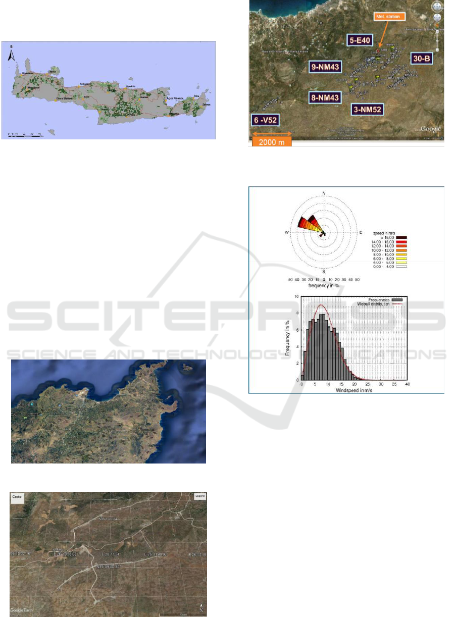
A rather large wind farm is located in a mountainous
area on the island of Crete, near the village of
Xirolimni (Figure 1,2). The wind farm has geographic
coordinates from N35 10 '12 "E26 08' to N35 07’ 48
"E26 14'. The wind farm was located on different
levels on mountain terrain and has different models
of Horizontal Axis Wind Turbine (HAWT) with
Power from 0.3 MW till 0.8 MW (Figure 3,4). Due to
the fact that the wind farm is located between the
major coastal cities in bay area Sitia, Hagia Photia
Strijhak, S., Koshelev, K. and Kryuchkova, A.
Investigation of Characteristics in Mountain Area with the Aim of Collecting Data for Modelling Flow Turbulent Parameters in a Wind Farm Located in a Coastal Area.
DOI: 10.5220/0007839803450353
In Proceedings of the 5th International Conference on Geographical Information Systems Theory, Applications and Management (GISTAM 2019), pages 345-353
ISBN: 978-989-758-371-1
Copyright
c
2019 by SCITEPRESS – Science and Technology Publications, Lda. All rights reserved
345
and Kato Zakros, it is necessary to assess the impact
of the wind farm and turbulent wakes on the local
microclimate of the region.
Figure 1: The map of the island of Crete.
The terrain orography data with the highest point of
745 meters was obtained using Google Earth Pro
software from Internet and satellite imagery. The
mountainous data were converted to the WGS 84
UTM 35N metric coordinate system using the QGIS
open source software package. The final surface of
the mountainous terrain near the village of Xirolimni
was constructed using asc file format transferred to
the STL format file, using in-house converter
program, according to the results of the collected data
on the coordinates of the complex terrain. As it was
shown by measurements based on the meteorological
tower data from the station, the wind was directed in
this region from north-west to south-east
(Kanellopoulos et al., 2013). The average wind
velocity was 8.5 meters per second (Figure 5).
Figure 2: The map of the east part for the island of Crete.
Figure 3: The map of the wind farm on the island of Crete.
Figure 4: The location of the wind turbines in the wind farm
on the island of Crete.
Figure 5: The data for velocity from Meteo station.
2.1 Mathematical Model
Large-Eddy Simulation approach (LES) using finite
volume method for the solution of the main equations
reflecting conservation laws was used. The following
equations are considered: the continuity equation (1),
the momentum equation (2), the transport of scalar
value - potential temperature equation (3) and other
equations (4)-(8).
The sub grid-scale models are an important part of
LES for Atmospheric Boundary Layer (ABL). The
SGS stress tensor was raised from the filtering of the
Navier-Stokes equations. The Boussinesq
approximation for buoyancy force is included with
the separate term in the momentum equation. The
final mathematical model included the following
equations (1-8).
ONM-CozD 2019 - Special Session on Observations and Numerical Modeling of the Coastal Ocean Zone Dynamics
346

(1)
(2)
3)
(4)
(5)
(6)
(7)
(8)
where,
is the resolved Cartesian velocity field, is
modified pressure variable, which is the density-
normalized deviation in resolved-scale static pressure
from its time-averaged value (in the absence of finite
time-averaged vertical gradients of temperature),
=
−
is the deviatoric part of the sub-grid-
scale (SGS) stress tensor and
is the SGS stress
tensor,
is the trace of the stress tensor.
is a
partially constant driving pressure gradient term used
to achieve a specified mean geostrophic wind,
is the
resolved virtual potential temperature,
is the
reference virtual potential temperature,
is the
gravity vector,
- is the alternating symbol,
is the
Coriolis parameter, and the subscripts 1, 2, and 3 refer
to the x-, y-, and z-directions, respectively.
is set
to the initial virtual potential temperature below the
capping inversion of 300K.
All physical quantities were defined in the centre of a
numerical volume cell. The features of a land
topography, influence of environment stratification,
Earth rotation, and change of thermal fluxes were
considered for flow parameters calculation.
Large-scale vortex structures were defined by
means of the filtered equations integration (Sagaut,
2010). The box filter was used for receiving the
filtered equations, the small eddies which size did not
exceed a step of a numerical grid were modelled by
means of a Lagrangian dynamic model of
Smagorinsky for subgrid turbulent viscosity - LASI
(Germano et al., 1991; Meneveau et al., 1996). An
additional model with restriction on dynamic
Smagorinsky constant value Cs was used to avoid its
negative values appearing during calculation
processes.
The terms in the equations (1-8) were
approximated with the first and second order of
accuracy on time and space. The obtained equations
for velocity, pressure, and potential temperature
coupling were solved by means of an iterative
algorithm PIMPLE. The procedure predictor-
corrector was realized for values of velocity, pressure,
and potential temperature as it was made in paper
(Oliveira and Issa, 2001). The obtained system of the
algebraic equations were solved by the iterative
method of conjugate gradients with a preconditioner
for velocity, pressure, potential temperature, stress
tensor and parameters of the turbulence subgrid scale
model. The total quantity of the calculated physical
values (scalar, vector and tensor) depending on the
selected turbulence model for subgrid scale viscosity
can be from 25 to 33. In this regard the resources of
High Performance Computing (HPC), or
supercomputer are required.
The surface shear-stress model was calculated
using Schumann model (Schumann, 1975). The stress
tensor components are equal to zero on the surface,
except values R13, R23.
Average and fluctuation values fields (velocity,
pressure, potential temperature, sub grid viscosity,
stress tensor, a thermal fluxes and others) were
obtained during calculation. The ABL Solver as a part
of open source library OpenFOAM 2.4 in the parallel
mode was used for final modelling of parameters in
turbulent flow (Churchfield et al., 2010; 2012).
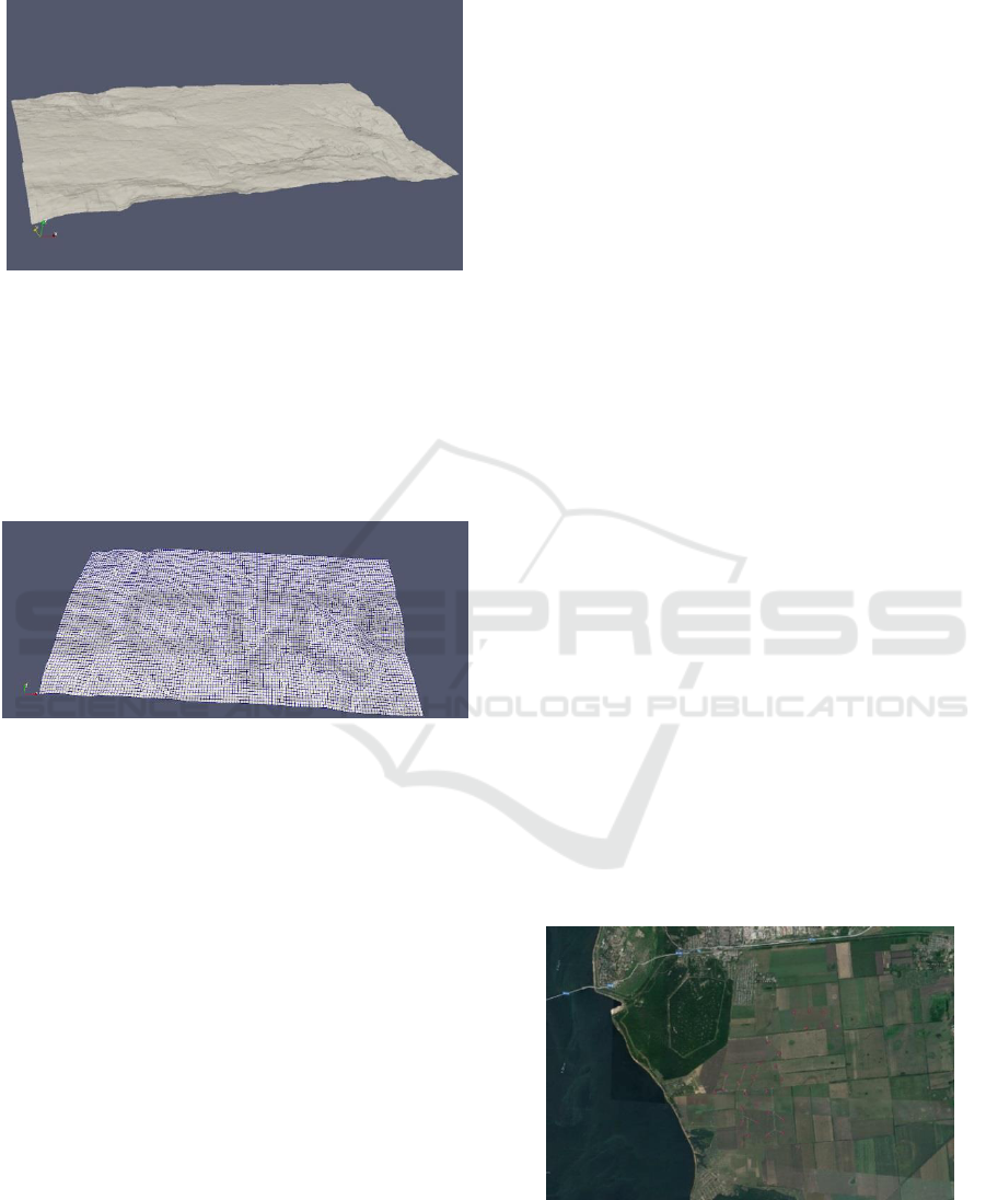
2.2 Formulation of the Problem
A computational domain with dimensions of 9.4 km
x 2.0 km x 4.6 km in the x-, y-, and z-directions was
chosen. The STL surface of complex terrain, which
was built using of Shuttle Radar Topography
Mission, for the region of wind farm near the village
of Xirolimni is shown in Figure 6.
The selected domain was periodic in the lateral
directions; the wall conditions were applied at the
lower surface; and a rigid, stress-free lid is used on
the top boundary. The atmospheric stability was set
to neutral with the potential temperature initialized
with value of 300K along the height of 1000m above
the surface. A strong capping inversion is applied in
Investigation of Characteristics in Mountain Area with the Aim of Collecting Data for Modelling Flow Turbulent Parameters in a Wind Farm
Located in a Coastal Area
347
which the temperature rises to 308K in the next 1000
m.
Figure 6: The STL surface for the complex terrain.
The mesh was initially created with uniform
resolution using OpenFOAM blockMesh tool, and
then OpenFOAM snappyHexMesh tool was used to
create the 3D unstructured grid representing the real
terrain. Various grids were considered with following
number of cells: a) 265 200; b) 520 000; c) 2 200 000
(Figure 7).
Figure 7: The mesh for the complex terrain.
The final simulation domain was defined by
dimensions: 9000 meters x 4300 meters x 2000
meters in width (x-), transverse (y-), and height (z-)
directions.
The simulation of the flow around mountainous
terrain can be performed using the ABLSolver solver
developed as a part of SOWFA open-source library.
SOWFA (Simulator for On/Offshore Wind Farm
Application) open-source library is based on
OpenFOAM. It includes several incompressible
solvers and utilities, it was developed in NREL, USA,
and now is of active use by the research community
(Churchfield et al., 2010; 2012).
Neutral Atmospheric Boundary Layer (ABL) case
with a given latitude was considered, the simulation
takes place at 35
o
north latitude. A logarithmic
velocity profile can be specified with a maximum
value of 8.5 meters per second at the inlet of the
computational domain. Fields of velocity,
temperature, pressure, turbulent subgrid viscosity
were of interest as a result of the calculation using the
Large Eddy Simulation method and dynamic
Smagorinsky model for turbulent subgrid viscosity.
The calculation should be done for t=20 000 seconds
to take into account both night-time and day-time
physical processes.
3 WIND FARM WITH FLAT
TERRAIN IN RUSSIA
The wind energy industry development in Russian
Federation involves designing and operation of new
wind power plants and turbines. Wind farms can
operate in various climatic conditions on the large
territory of the country (Ulyanovsk oblast, Republic
of Adygea, Taman Peninsula, Arctic region). A new
wind farm was built recently in Ulyanovsk region of
Russian Federation (RF) in 2017, 2018 years (Figure
8). The wind farm has geographic coordinates N54
o
17 ' E48
o
08'.
Similar studies were conducted for the 3D region
corresponding to the ABL and the model wind farm
with 2 and 12 wind turbines (Tellez-Alvarez et al.,
2017, Kryuchkova et al., 2017, Strijhak et al., 2018).
The ABL calculations for the area including wind
farm in Ulyanovsk oblast of RF were carried out in a
spatial area of 3km x 3km x 1.02km in size on
numerical grids 150x150x51 and 300x300x102
during time of 20000 seconds (Tellez-Alvarez et al.,
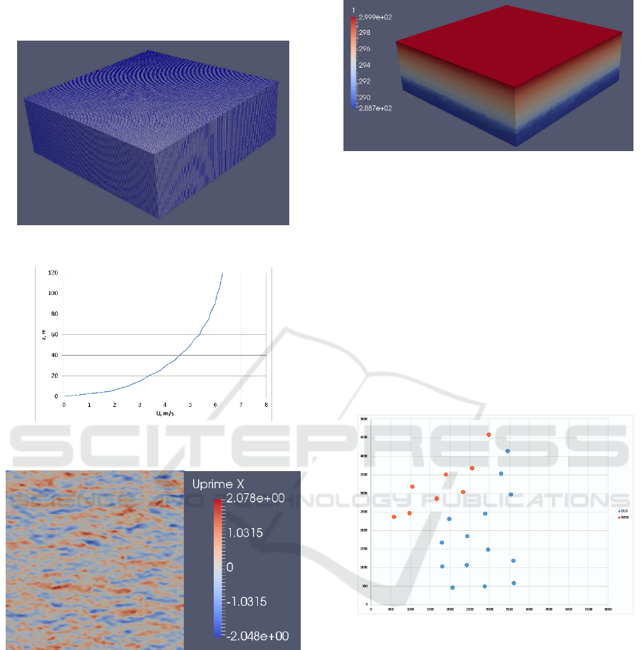
2017). The 3D numerical domain and grid are shown
in Figure 9. The inlet velocity profile which is taken
from field measurements is shown on Figure 10. The
value of aerodynamic roughness height z0
was set to
0.1. The streamwise velocity fluctuations at 90 m
above the surface for the case using numerical mesh
150 x 150 x 51 are shown in Figure 11. These
fluctuations values can reach about 25% of the mean
velocity value.
Figure 8: The territory of wind farm near the Volga River.
It is necessary to take these velocity and pressure
fluctuations into account in case of physical
ONM-CozD 2019 - Special Session on Observations and Numerical Modeling of the Coastal Ocean Zone Dynamics
348
parameters simulations of large wind turbines in wind
farms.
Figure 9: The 3D numerical domain for ABL case.
Figure 10: The inlet velocity profile for ABL case.
Figure 11: The streamwise velocity fluctuations at 90 m.
The mean potential temperature field is shown in
Figure 12. Cooling ground and heating the upper
layer produce internal waves dominated by the Brunt-
Vaisala frequency. The obtained data from ABL
simulation (Figure 11, 12) can be used for further
studies of wind farms with model wind turbines of
different power (Figure 13). The orography of the
area can be also taken into account and the impact of
the wind farm and turbulent wakes on the local
microclimate of the area can be assessed.
Figure 12: The temperature field for 3 D domain.
3.1 Formulation of the Problem
An additional investigation was done for the case of
wind farm in Ulyanovsk oblast RF, Krasny Yar
(Figure 8).
It is known that the Reynolds numbers can reach
order of Re=10e7-10e8 considering the characteristic
sizes of wind turbine blades. It is difficult to resolve
all flow scales by means of LES since too big
numerical grids would be required for this purpose.
It is well-known that Actuator Line Model (ALM)
approach doesn't demand too detailed grids around
the turbine blades.
Figure 13: The wind farm with 28 wind turbines.
This approach allows to represent various types of
vortexes, wake, trailer, root and boundaries vortexes.
In the scope of ALM turbine blades are approximated
by separate flat sections with a given profile, chord,
and twist. The values of lift and drag forces are
collected in tables for each profile. The force
projected on the flow is equal to the aerodynamic
force applied on operating turbine blades. The
procedure of force projection comes to a number of
separate terms adding in the momentum equation.
The resultant force is determined with following
technique:
Investigation of Characteristics in Mountain Area with the Aim of Collecting Data for Modelling Flow Turbulent Parameters in a Wind Farm
Located in a Coastal Area
349
(9)
Where
is actuator point force projected as a
body force onto Computational Fluid Dynamics
(CFD) grid, where is the distance between CFD
cell center and actuator point, is Gaussian filter
width related to the initial intermittency. The
term was added as additional term in the
momentum equation 2. The further details of this
procedure can be found in (Sørensen and Shen, 2002).
The Gauss linear Scheme was used for approximation
of the convective terms, the Gauss linear corrected
scheme was used for approximation of laplacian
terms. To solve linear system equations the PBiCG
method with DILU preconditioner was used for
velocity, temperature and the GAMG method was
used for pressure. The tolerance was set to 1e-6.
The first 14 wind turbines in model wind farm
were considered in case with SOWFA library (Figure
13).
The diameter of rotor for wind turbine was equal
to D=416 mm. The reference velocity was set to
Uref=1.5 m/s. Atmospheric Boundary Layer model
was introduced to represent experimental conditions.
The parameters of Neutral ABL, used in our
simulation, are listed in Table 1 of work (Hancock
and Farr, 2014).
Each of the prototype wind turbines had 3 blades
with constant cross section. The blade was made of
carbon fibre with a shape of a twisted thin flat plate
of 0.8 mm thickness, without using any aerofoil
cross-section (Hancock and Farr, 2014). Operating
tip-speed ratio (TSR) was set to 6.
The ABLSolver and pisoFoamTurbine solvers
allow distinguishing the mean and turbulent wake
flows behind turbines in series and the behaviour of
the whole turbines array. The simulation was run in
3D box domain.
The pisoFoamTurbine solver was tested on famous
Blind Test 2 with two turbines (Kryuchkova et al.,
2017; Strijhak et al., 2017; Pierella et al., 2014).
The domain with following dimensions was
selected: 6500 mm x 5500 mm x 1000 mm in width
(x-), transverse (y-), and height (z-) directions.
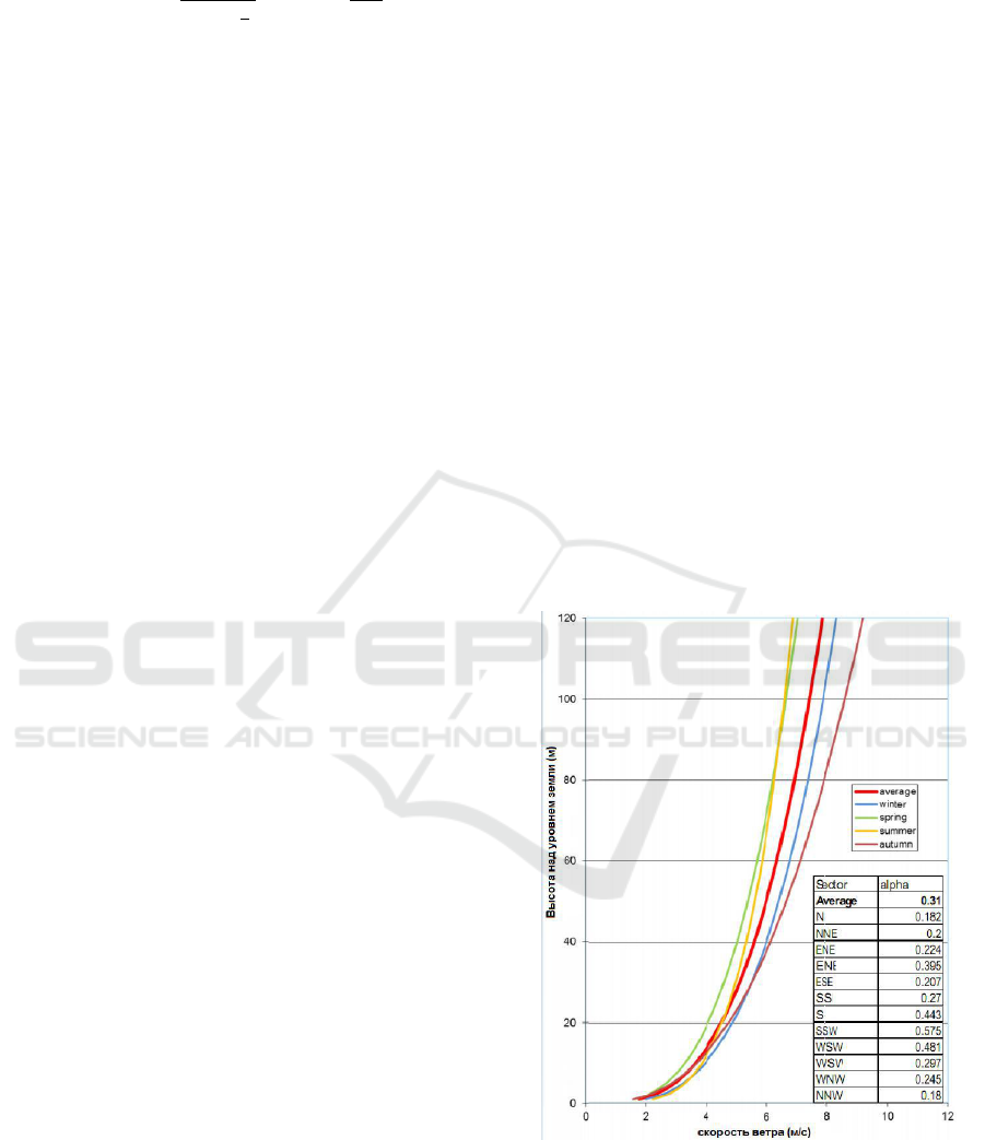
The data on velocity profile and wind direction were
taken from the weather station and the free report of
Lahmeyer International Company in Internet for the
period of time from 26.05.2012 till 25.05.2013
(Figure 14-Figure 16).
The wind was directed in this area from north-west
to south-east, and the average wind speed was 6.5
meters per second.
The numerical technique comprised a preliminary
simulation with ABLSolver aimed to define the inlet
parameters for the major domain with rotating wind
turbines, the second step consisted in numerical
simulations using pisoFoamTurbine.
This method is called in literature as a “Precursor”
method for LES (Figure 17) (Churchfield et al.,
2012).
The value of numBladePoints for the case with 14
wind turbines was set to 40, the epsilon value was set
to 5.0 in Formula 9.
The resulting unstructured mesh for the test with
14 wind turbines counted 2 millions of cells.
After constructing the primary mesh with
blockMesh tool the central zone with the turbines
array inside was refined twice and an additional
refinement was done around each turbine. The final
mesh had 6 millions of cells.
The small eddies for which the size didn't exceed
grid cell size were modelled by means of the
Lagrangian-averaged scale-independent dynamic
Smagorinsky model (Meneveau et al., 1996).
Figure 14: The velocity profile in wind farm of Ulyanovsk
oblast of RF.
ONM-CozD 2019 - Special Session on Observations and Numerical Modeling of the Coastal Ocean Zone Dynamics
350
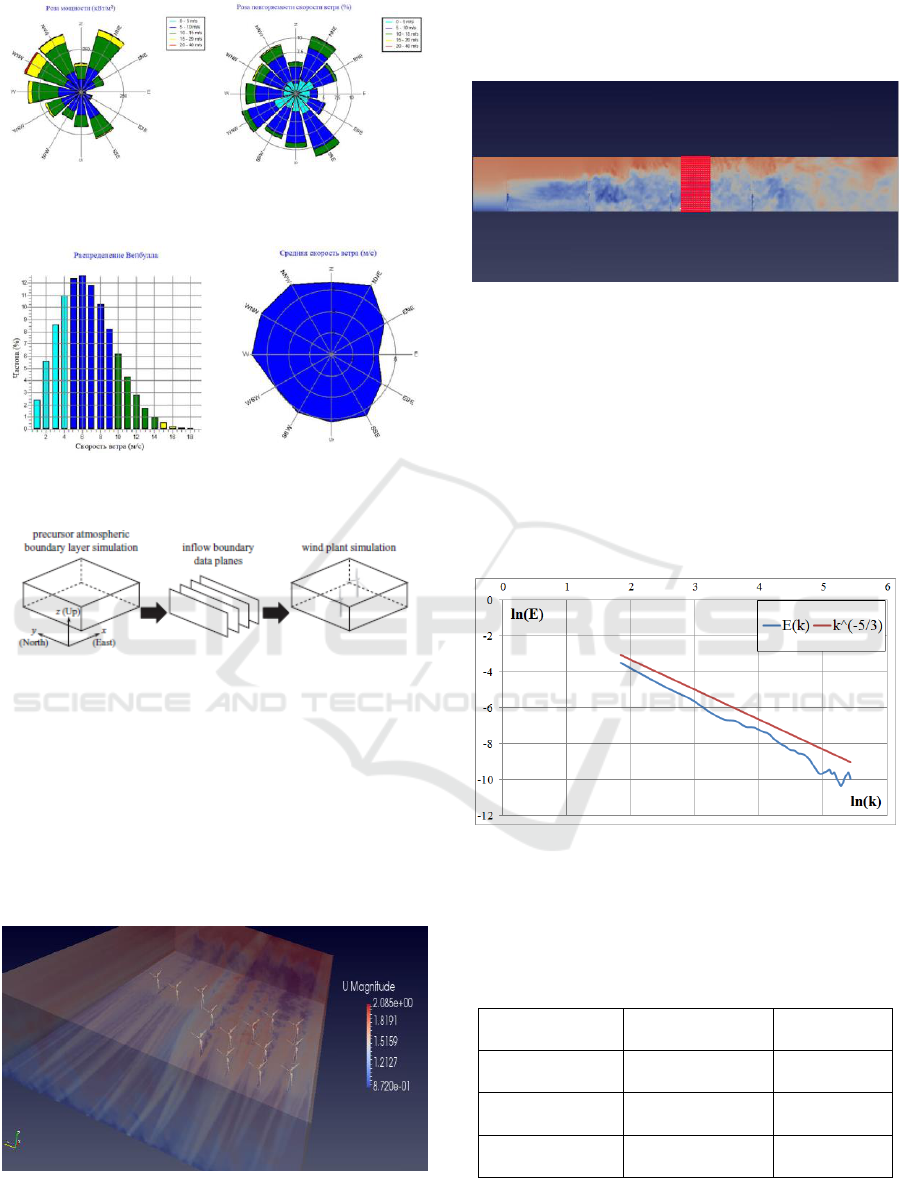
Figure 15: The wind rose in wind farm of Ulyanovsk oblast
of RF.
Figure 16: The Weibull distribution and average velocity in
wind farm of Ulyanovsk oblast of RF.
Figure 17: The procedure of “Precursor” method.
3.2 Results of Simulation
The flow patterns around four turbines aligned to the
first row of the array were studied to determine the
general behaviour of the resulting flow in the model
wind farm. It was noted that the wakes behind the first
turbines row are more stable, but with the second and
the third turbine’s rows the wake turbulent behaviour
becomes more pronounced (Figure 18).
Figure 18: The numerical domain for wind farm simulation
with 14 model wind turbines.
In order to study the value of the Energy Spectrum
of turbulence E(k) with FFTW library a 3D box
comprising an even mesh was created (Figure 19).
Figure 19: 3D box in numerical domain for calculation
E(k).
The velocity field was then interpolated into the
box and FFTW 3.3.8 library was applied. The
calculated Energy Spectrum E(k) in Fourier space
was closed to Kolmogorov-Obukhov k-5/3 spectrum
and is shown on Figure 20 (Pope, 2000).
The calculations were carried out on the high
performance computer cluster of ISPRAS in web-
laboratory UNICFD using 12-72 computer cores for
each numerical case.
Figure 20: The Energy Spectrum E(k).
The simulation results for a model wind farm with 14
wind turbines for physical time t=1.0 second are
presented in Table 1.
Table 1: The results of simulations.
Number of
processors
Execution time
(seconds)
Speedup
12 cores in 1
computer node
27650
-
36 cores in 3
computer nodes
9104
3.04
72 cores in 6
computer nodes
5842
4.73
Investigation of Characteristics in Mountain Area with the Aim of Collecting Data for Modelling Flow Turbulent Parameters in a Wind Farm
Located in a Coastal Area
351

4 CONCLUSIONS
We have used SOWFA library and ABLSolver solver
to setup a case for ABL simulation with the complex
mountain terrain for wind farm located in Crete near
the village of Xirolimni. A LES simulation with a flat
terrain using various solvers of SOWFA library was
carried out for the Russian wind farm located in
Ulyanovsk oblast RF. In connection with the small
size of the wind turbines and the large velocity of
blades rotation we can neglect some terms like the
horizontal gradient of pressure and Coriolis force in
momentum equation. This approach allows us to take
into account the orography of the area, different
physical processes in ABL like lower-level jets (Basu
et al., 2010; Baas et al., 2009), large scale motions and
vortices (Huang et al.,2009; Shah and Bou-Zeid,
2014), structure functions, scaling exponents and
intermittency in turbulent wakes (Vindel, et al., 2008;
Ali, et al., 2016). The method makes possible
modelling of turbulent boundary layer flow over
fractal-like multiscale terrain using LES (Yang and
Meneveau, 2017) and assessing the impact of the
wind farm and turbulent wakes on the local
microclimate of the region.
ACKNOWLEDGEMENTS
The authors wish to acknowledge the financial
support from Russian Foundation of Basic Research -
RFBR (Grant No. 17-07-01391).
REFERENCES
Mehta, D., et al. 2014. Large eddy simulation of wind farm
aerodynamics: a review. Journal of Wind Energy &
Industrial Aerodynamics, 133, pp.1–17.
Stevens, R.J.A.M., Meneveau, C., 2017. Flow Structure and
Turbulence in Wind Farms. Annual Review of Fluid
Mechanics, 49, pp. 311–39.
Tsoutsos, T., et al., 2015. Sustainable siting process in large
wind farms case study in Crete. Renewable Energy, 75,
pp. 474-480.
Kanellopoulos, D., et al., 2013. The Cretan wind farms.
Estimating Energy Output in Areas of complex terrain.
Conference of the Wind Power Engineering
Community. Berlin, Germany, 18–19 June 2013.
Sagaut, P. 2002. Large eddy simulation for incompressible
flows: an introduction, Berlin. Springer.
Germano, M., Piomelli, U., Moin, P., Cabot, W. H., 1991.
A dynamic subgrid-scale eddy viscosity model. Phys.
Fluids, 3, pp. 1760–1765.
Meneveau, C., Lund, T. S., Cabot, W. H., 1996. A
Lagrangian dynamic subgrid-scale model of
turbulence. J Fluid. Mech, 319, pp. 353–385.
Oliveira, P. J., Issa, R. I., 2001. An improved PISO
algorithm for the computation of buoyancy-driven
flows. Numerical Heat Transfer, 40 (B), pp. 473-493.
Schumann, U., 1975. Subgrid-Scale Model for Finite-
Difference Simulations of Turbulent Flow in Plane
Channels and Annuli. Journal of Computational
Physics, 18, pp. 76–404.
Churchfield, M. J., Moriarty, P. J., Vijayakumar, G.,
Brasseur, J. G., 2010. Wind Energy-Related
Atmospheric Boundary Layer Large-Eddy Simulation
Using OpenFOAM. 19th Symposium on Boundary
Layers and Turbulence. Keystone, Colorado, USA, 2 -
6 August 2010. NREL.
Churchfield, M. J., Lee. S., Michalakes, J., Moriarty. P. J.,
2012. A numerical study of the effects of atmospheric
and wake turbulence on wind turbine dynamics.
Journal of Turbulence, 13(14), pp. 1–32.
Tellez-Alvarez, J., Koshelev, K., Strijhak, S., Redondo,
J.M., 2019. Simulation of turbulence mixing in
atmosphere boundary layer and analysis of fractal
dimension. Physica Scripta, [e-journal].
https://doi.org/10.1088/1402-4896/ab028c.
Kryuchkova, A., Tellez-Alvarez, J., Strijhak, S., Redondo
J.M., 2017. Assessment of Turbulent Wake Behind
Two Wind Turbines Using Multi-Fractal Analysis.
Ivannikov ISPRAS Open Conference (ISPRAS).
Moscow, Russia, 30 November – 1 December 2017.
IEEE. https://doi.org/10.1109/ISPRAS.2017.00025
Strijhak, S.V., Koshelev, K.B., Kryuchkova, A.S., 2018.
Studying parameters of turbulent wakes for model wind
turbines. AIP Conference Proceedings, [e-journal]
2027, 030086 (2018). pp. 1-8.
https://doi.org/10.1063/1.5065180.
Sørensen, J.N., Shen, W.Z., 2002. Numerical Modelling of
Wind Turbine Wakes. Journal of Fluids Engineering,
124, pp.393-399.
Hancock P.E., Farr T.D., 2014. Wind-tunnel simulations of
wind-turbine arrays on neutral and non-neutral winds.
J. Phys.: Conf. Ser., 524 012166.
Hancock, P.E., Pascheke, F., 2014. Wind-Tunnel
Simulation of the Wake of a Large Wind Turbine in a
Stable Boundary Layer: Part 2, the Wake Flow.
Boundary-Layer Meteorology, 151, pp. 23–37.
Pierella, F., Krogstad, P.A., Sætran, L., 2014. Blind Test 2
calculations for two in-line model wind turbines where
the downstream turbine operates at various rotational
speeds. Renewable Energy, 70, pp. 62–77.
Pope S.B., 2000. Turbulent Flows, Cambridge. Cambridge
University Press.
Basu, S. et al., 2010. Stable boundary layers with lower-
level jets: what did we learn from the LES
intercomparison within GABLS3? The Fifth
International Symposium on Computational Wind
Engineering (CWE2010). Chapel Hill, North Carolina,
USA, 23-27 May 2010. pp. 1-8.
Baas, P., Bosveld, F.C., Klein Baltink, H., and Holtslag,
A.A.M., 2009. A climatology of nocturnal low level jets
ONM-CozD 2019 - Special Session on Observations and Numerical Modeling of the Coastal Ocean Zone Dynamics
352

at Cabauw. Journal of Applied Meteorology and
Climatology, 48, pp. 1627-1642.
Huang, J., Cassiani, M., Albertson, J. D., 2009. Analysis of
coherent structures within the atmospheric boundary
layer. Boundary-Layer Meteorology, 131, pp. 147–171.
Shah, S., Bou-Zeid, E., 2014. Very-Large-Scale Motions in
the Atmospheric Boundary Layer Educed by Snapshot
Proper Orthogonal Decomposition, Boundary-Layer
Meteorology, 153 (3), pp. 355-387.
Vindel, J.M., Yage, C., Redondo, J.M., 2008. Structure
function analysis and intermittency in the atmospheric
boundary layer. Nonlinear Processes Geophys., 15, pp.
915-929.
Ali, N., Aseyev, A.S., Cal R.B., 2016. Structure functions,
scaling exponents and intermittency in the wake of a
wind turbine array. Journal of renewable and
sustainable energy, 8, pp. 013304-1 - 013304-9.
Yang, X.I.A., Meneveau, C. 2017. Modelling turbulent
boundary layer flow over fractal-like multiscale terrain
using large-eddy simulations and analytical tools. Phil.
Trans. R. Soc. A., 375, 20160098. pp.1-19.
https://doi.org/10.1098/rsta.2016.0098.
Investigation of Characteristics in Mountain Area with the Aim of Collecting Data for Modelling Flow Turbulent Parameters in a Wind Farm
Located in a Coastal Area
353
