An Evaluation between Global Appearance Descriptors based on

Analytic Methods and Deep Learning Techniques for Localization in

Autonomous Mobile Robots

Sergio Cebollada

, Luis Pay

, David Valiente

, Xiaoyi Jiang

and Oscar Reinoso

Department of Systems Engineering and Automation, Miguel Hern

andez University, Elche, 03202, Spain

Department of Computer Science, University of M

unster, M

unster, 48149, Germany

Keywords:

Mobile Robots, Omnidirectional Images, Global Appearance Descriptors, Localization, Deep Learning.

Abstract:

In this work, different global appearance descriptors are evaluated to carry out the localization task, which is

a crucial skill for autonomous mobile robots. The unique information source used to solve this issue is an om-

nidirectional camera. Afterwards, the images captured are processed to obtain global appearance descriptors.

The position of the robots is estimated by comparing the descriptors contained in the visual model and the

descriptor calculated for the test image. The descriptors evaluated are based on (1) analytic methods (HOG

and gist) and (2) deep learning techniques (auto-encoders and Convolutional Neural Networks). The localiza-

tion is tested with a panoramic dataset which provides indoor environments under real operating conditions.

The results show that deep learning based descriptors can be also an interesting solution to carry out visual

localization tasks.

1 INTRODUCTION

Nowadays, the use of visual information to solve mo-

bile autonomous robotic tasks is widely expanded.

In these cases, the robot must be able to build a

map within the environment and estimate its position

within that environment. These tasks are known as

mapping and localization. Among the different sen-

sors used, the omnidirectional cameras introduce an

interesting solution since they are able to provide in-

formation that covers a ﬁeld of view of 360 deg.

Global appearance descriptors have been pro-

posed by several authors to extract characteristic in-

formation from images and use this information for

mapping and localization. For instance Zhou et

al. (Zhou et al., 2018) propose the use of the de-

scriptor gist to solve the localization through match-

ing the best keyframe in the dataset based on the given

robot’s current view. Korrapati and Mezouar (Korrap-

ati and Mezouar, 2017) introduced the use of omnidi-

rectional images through global appearance descrip-

tors to create a topological mapping approach and a

loop closure detection method. More recently, Rom

et al. (Rom

an et al., 2018) evaluate the use of global

appearance descriptors for localization under illumi-

nation changes. In this work, several distance mea-

surements were also evaluated with the aim to obtain a

similitude distance between images which represents

the geometrical distance between the positions where

those images were captured.

The computation of these descriptors is based on

analytic methods, nevertheless, during the last years,

some authors have proposed the use of deep learn-

ing techniques to create global appearance descrip-

tors. For example, on the one hand, Xu et al. (Xu

et al., 2016) proposed the use of auto-encoders to de-

tect histopathological images of breast cancer. On the

other hand, Xu et al. (Xu et al., 2019) used a CNN-

based descriptor to obtain the most probable position

within an indoor map through Monte Carlo Localiza-

tion and also to solve the kidnapping problem; Pay

et al. (Pay

a et al., 2018) proposed also the use of

the CNN-based descriptors but in this case for hier-

archical mapping. Both works are based on the net

places (Zhou et al., 2014). The descriptors extracted

from this network correspond to the ones calculated

in some of the fully convolutional layers within the

network.

Through this work, we carry out a comparison

between global appearance descriptors based on an-

alytic methods and global appearance descriptors

based on deep learning techniques to solve the visual

localization task. The goodness of these methods are

measured according to the accuracy (error of localiza-

284

Cebollada, S., Payá, L., Valiente, D., Jiang, X. and Reinoso, O.

An Evaluation between Global Appearance Descriptors based on Analytic Methods and Deep Learning Techniques for Localization in Autonomous Mobile Robots.

DOI: 10.5220/0007837102840291

In Proceedings of the 16th International Conference on Informatics in Control, Automation and Robotics (ICINCO 2019), pages 284-291

ISBN: 978-989-758-380-3

tion) and computing time (to calculate the descriptor

and to estimate the position of the robot).

The remainder of the paper is structured as fol-

lows: Section 2 explains the algorithm used to esti-

mate the position of the test images within the en-

vironment. After that, section 3 outlines the global

appearance descriptors which will be evaluated. Sec-

tion 4 explains and presents the dataset used as well

as the experimental results and the discussion about

them. Finally, section 5 outlines the conclusions and

future research lines.

2 LOCALIZATION METHOD

The localization task consists in an image retrieval

problem. This is, obtaining the image which presents

higher similitude in relation to the new captured im-

age. For this purpose, the robot has previously ob-

tained visual information from the environment, i.e.,

global appearance descriptors that are calculated from

the N

Train

images captured from different positions of

the environment. This task is known as mapping and

this step must be carried out before starting the lo-

calization. Therefore, the localization task is solved

through the following steps:

• The robot captures a new omnidirectional image

from an unknown position.

• That image is transformed to panoramic (im

test

)

and after that, the corresponding descriptor is cal-

culated (

test

• Once the descriptor is available, the robot cal-

culates the cosine distance (selected in (Cebol-

lada et al., 2019) as the best distance method for

global appearance descriptors) between the test

descriptor (

test

) and each descriptor from the vi-

sual model (

, where j = 1, ..,N

Train

• A vector of distances is obtained as

,..., h

Train

} where h

t j

= dist{

test

• The node which presents the minimum

distance(d

|t = argmin

t j

) corresponds to

the estimated position of the robot.

3 THE GLOBAL APPEARANCE

DESCRIPTORS

Visual localization has been commonly solved either

using local features along a set of scenes or using a

unique descriptor per image which contains informa-

tion on its global appearance. These second methods

are know as global appearance description and have

been used to solve the localization task since they al-

low straightforward localization algorithms. For in-

stance, Naseer et al. (Naseer et al., 2018) propose a

localization method from global appearance (by us-

ing histogram of oriented gradients descriptors and

features from deep convolutional neural networks) to

solve the localization problem and to keep in parallel

several possible trajectories hypotheses.

Basically, the steps to calculate a global appear-

ance descriptor are the following: (1) The starting

point is a panoramic image expressed as a bidirec-

tional matrix (im

∈ R

×M

). (2) Then the speciﬁc

mathematical calculations are applied and a vector

which characterizes the original image will be ob-

tained (

∈ R

l×1

and corresponds to the image im

The ﬁrst global appearance descriptors used in

computer vision were descriptors based on analytic

methods. Nevertheless, during the last years, the

emergence of the deep learning techniques have em-

powered the use of descriptors based on these new

methods.

3.1 Methods based on Analytic Methods

These methods are basically based on calculations of

gradients and orientation of the different pixels which

compose the image. Their use has been quite often

to solve mobile robotics issues. For instance, Su et

al. (Su et al., 2017) used a global descriptor to reduce

pose search space with the aim to solve the kidnapped

robot problem in indoor environments under different

conditions. An interesting study was carried out by

Rom

an et al. (Rom

an et al., 2018) which evaluates

the use of global appearance descriptors for localiza-

tion under illumination changes. More recently, Ce-

bollada et al. (Cebollada et al., 2019) evaluate the use

of global appearance descriptors to build hierarchical

maps through clustering algorithms and then to solve

the localization in those maps.

Among the different methods, this work proposes

the use of HOG and gist, which have been used in pre-

vious works (Cebollada et al., 2019) and have proved

to present interesting results for localization tasks.

Regarding the HOG descriptor, it was introduced

by Dalal and Triggs (Dalal and Triggs, 2005) to

solve the detection of pederastians. In this work,

the procedure is the one proposed by Leonardis

and Bischof (Leonardis and Bischof, 2000): the

panoramic image is divided into k

horizontal cells

and a histogram of gradient orientation (with b bins

per histogram) is compiled per each cell. Finally, the

set of histograms are arranged in a unique row to com-

pose the ﬁnal descriptor

d ∈ R

b·k

×1

An Evaluation between Global Appearance Descriptors based on Analytic Methods and Deep Learning Techniques for Localization in

Autonomous Mobile Robots

285

As for the gist descriptor, it was introduced by

Oliva et al. (Oliva and Torralba, 2006). In this work,

the version used consists on: (1) obtaining m

dif-

ferent resolution images, (2) applying Gabor ﬁlters

over the m

images with m

different orientations,

(3) grouping the pixels of each image into k

hori-

zontal blocks and (4) arranging the obtained orien-

tation information into one row to create a vector

d ∈ R

·m

·k

×1

3.2 Methods based on Deep Learning

During the last years, the use of deep learning meth-

ods to solve computer vision issues has extensively

grown. Regarding the localization task through the

use of visual information, this work studies the use of

Convolutional Neural Networks (CNN) and the use

of auto-encoders. The idea is to obtain vectors which

characterize the images through some deep learning

technique. On the one hand, these methods can re-

sult very interesting since their use can be focused on

speciﬁc kind of images (such as indoor environments

in our case) and, hence, providing more efﬁcient de-

scriptors. On the other hand, these methods lead to

previous training which normally implies huge pro-

cessing data and noteworthy time.

Regarding the use of CNNs, these networks have

been commonly designed for classiﬁcation. In this

sense, (1) a set of images correctly labeled are col-

lected and introduced into the network to tackle the

learning process and after that, (2) the network is

properly available to face the classiﬁcation (test image

as input and the CNN outputs the most likely label op-

tion). The CNNs are composed by several hidden lay-

ers whose parameters and weights are tuned through

the training iterations. In this work, some hidden lay-

ers outputs are used to obtain global appearance de-

scriptors. This idea have already been proposed by

some authors such as Mancini et al. (Mancini et al.,

2017), who use them to carry out place categorization

with the Na

ıve Bayes classiﬁer or Pay

a et al. (Pay

et al., 2018), who proposed CNN-based descriptors

to create hierarchical visual models for mobile robot

localization. The CNN architecture that has been used

in this work is places (Zhou et al., 2014), which was

trained with around 2.5 million images to categorize

205 possible kinds of scenes (no re-training is carried

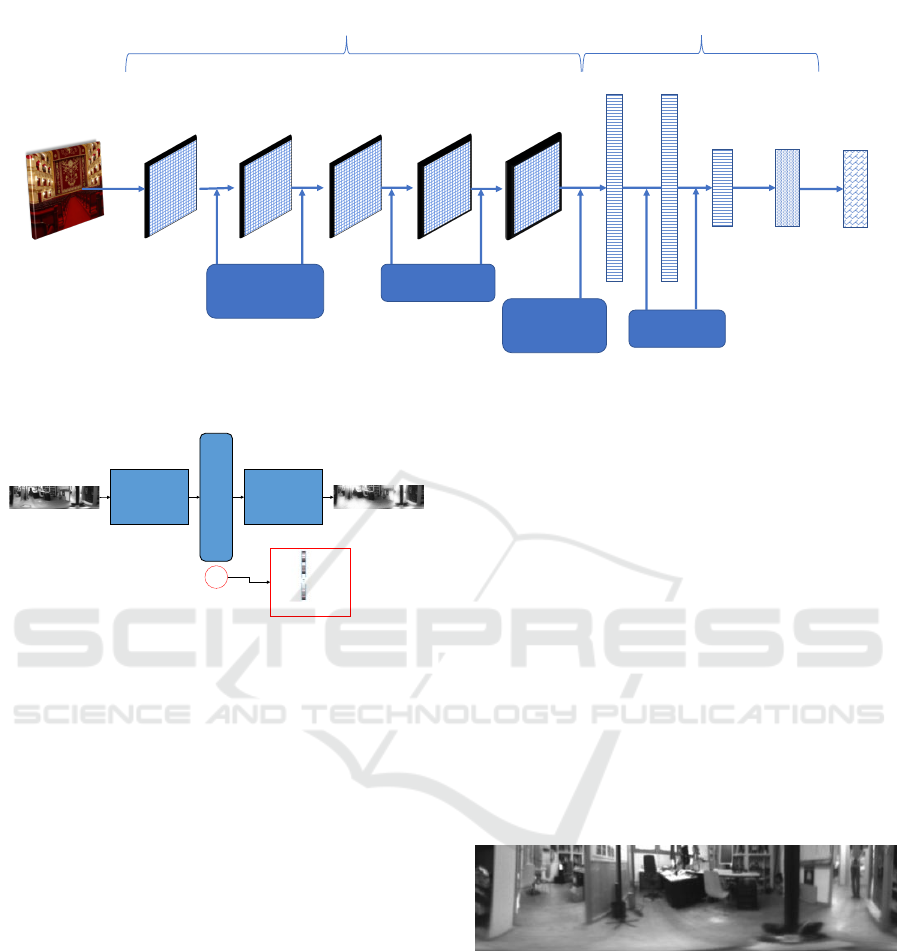
out in this work). Fig. 1 shows the architecture of

the places CNN, which is based on the caffe CNN.

The net basically consists in (1) an input layer, (2)

several intermediate hidden layers and (3) an output

layer. Within the intermediate layers, the ﬁrst phase

consists in (2.1) layers for featuring learning (whose

layers incorporate several ﬁlters and the output gen-

erated are used as input for the next layer) and (2.2)

layers for classiﬁcation (whose layers are fully con-

nected and they generate vectors which provide infor-

mation for classiﬁcation).

In this work, we have evaluated the output infor-

mation from 5 layers. Three fully convolutional layers

(’fc6’, ’fc7’ and ’fc8’) whose output size are 4096 ×1,

4096×1 and 205×1 respectively. Moreover, we have

obtained two descriptors from the output of 2D con-

volution layers (’conv4’ and ’conv5’). These layers

apply several sliding convolutional ﬁlters to the input

images with the aim to activate certain characteristics

of the image. Hence, the output of these layers is a set

of images which are the input image after being ﬁl-

tered. Finally, a descriptor is basically obtained from

these layers through selecting an image from the out-

put dataset and arranging the data (matrix) in a single

row (vector). Since the size of the output images is

13 × 13, the size of the descriptor is 169 × 1.

As for the use of auto-encoders, the aim of these

neural networks is to reconstruct the output through

compressing the input into a latent-space representa-

tion (Hubens, 2018). The ﬁg. 2 shows the architecture

design of the auto-encoders. These networks ﬁrstly

compress the input (encoding) and secondly recon-

struct the input departing from the latent space rep-

resentation (decoding). The idea consists in building

a latent representation to obtain useful features with

small dimension, i.e., training the auto-encoder to ex-

tract the most salient features. For example, Gao and

Zhang (Gao and Zhang, 2017) used auto-encoders

to detect loops for visual Simultaneous Localization

And Mapping (SLAM).

For this experiment, two types of auto-encoder

are proposed. Both have been trained using the

same parameters (Coefﬁcient for the L

weight reg-

ularizer, 0,004; Coefﬁcient that controls the impact

of the sparsity regularizer, 4; Desired proportion of

training examples a neuron reacts to, 0.15; Encoder

Transfer Function, “Logistic sigmoid function”; and

Maximum number of training epochs, 1000) and

also both have been trained using a GPU (NVIDIA

GeForce GTX 1080 Ti), but whereas the ﬁrst option

(auto-enc-Frib) is trained with the images obtained

from the dataset used to evaluate the localization (ex-

plained in sec. 4), the second alternative (auto-enc-

SUN) is trained with images obtained from a dataset

(SUN 360 DB (Xiao et al., 2012)) which contains

generic panoramic images. The aim of this second

option is to create a generic auto-encoder based on

indoor panoramic images which provides a good-

enough solution to obtain descriptors for panoramic

images independently the environment. This solution

would solve the handicap that introduces the descrip-

ICINCO 2019 - 16th International Conference on Informatics in Control, Automation and Robotics

286

RELU

Max pooling

RELU layer

RELU

Max pooling

RELU layer

Input

Image

227x227x3

C1-96

11x11

C2-256

5x5

C3-384

3x3

C4-384

3x3

C5-256

3x3

FC6

1x4096

FC7

1x4096

FC8

1x205

Softmax

Classification

output layer

FEATURE LEARNING CLASSIFICATION

Figure 1: CNN architecture design of the pre-trained ’caffe’ model.

Encoder

(



)

h=f(x)

Decoder

(



)

r=g(h)

Latent

Representation

Input

Reconstructed

Output

⃗





(



x1)

Figure 2: Auto-encoder architecture design and extraction

of features departing from the latent representation.

tor based on auto-encoders regarding the need to carry

out a previous training before calculating the descrip-

tors. For auto-enc-Frib, the training dataset consists

in 519 panoramic images whose size is 512 × 128;

for auto-enc-SUN, the training dataset consists in 541

panoramic images whose size is also 512 × 128. Fur-

thermore, the auto-encoders are trained varying the

size of hidden representation of the auto-encoder (this

number is the number of neurons in the hidden layer)

and the resultant descriptor size obtained depends di-

rectly on that number (N

HiddenSize

× 1). Regarding

the computing time to train these auto-encoders, the

computer needs between 6 min and 2,94 hours, being

directly proportional to the number of neurons (the

more number of neurons there are, the more comput-

ing time is required).

4 EXPERIMENTS

4.1 Dataset

The experiments were carried out through the use

of the COLD dataset (Pronobis and Caputo, 2009),

which contains visual information along a trajectory.

It contains three indoor laboratory environments in

three cities (Freiburg, Saarbr

ucken and Ljubljana) and

three different illumination conditions. Nevertheless,

for the experiments purposes, only the images related

to the Freiburg environment were used and no illu-

mination changes have been considered, i.e., the im-

ages used were only captured under cloudy conditions

(during the light hours but the sunlight does not con-

siderably affect the shots). This lack of illumination

changes is due to the fact that this work is focused on

studying the goodness of the descriptors for localiza-

tion task, however, in future works, an extension to

study the illumination changes effects will be consid-

ered. This dataset includes changes in the environ-

ment such as people walking or position of furniture

and objects. An example of these dynamic conditions

can be seen in ﬁg. 3.

Figure 3: Panoramic image from COLD database.

Among the different paths, the red one was se-

lected for this experiment because it is the longest.

Afterwards, the images are split into two datasets:

training and test datasets. Training dataset is com-

posed by 519 images which present an average dis-

tance around 20 cm between an image and the follow-

ing one. The test dataset is composed by 2595 images

and the average distance between images is 4,10 cm.

The table 1 shows the information about the datasets

in detail.

An Evaluation between Global Appearance Descriptors based on Analytic Methods and Deep Learning Techniques for Localization in

Autonomous Mobile Robots

287

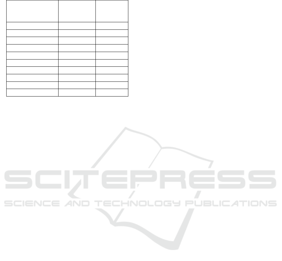
Table 1: Number of images in each room of the training and

test datasets created from the Freiburg environment.

Name

Number

of images

in Training

Number

of images

in Test

Printer area 44 223

Corridor 212 1044

Kitchen 51 255

Large Ofﬁce 34 175

2-persons ofﬁce 1 46 232

2-persons ofﬁce 2 26 131

1-person ofﬁce 31 154

Bathroom 49 247

Stairs area 26 134

Total number 519 2595

4.2 Evaluation of the Localization

To evaluate the goodness of each descriptor method

for localization, two parameters are considered: On

the one hand, (1) the average localization error, which

measures the Euclidean distance between the position

estimated and the real position where the test image

was captured. To obtain this value, the ground truth

provided by the dataset is used. Nevertheless, the

ground truth is only used for this purpose (it is not to

solve the localization task). On the other hand, (2) the

average computing time, which is analyzed through

two values, (2.a) the computing time to calculate the

descriptor and (2.b) the computing time to estimate

the position of the test image.

The results obtained through the use of ana-

lytic descriptors (HOG and gist) and the descriptors

based on deep learning (auto-encoders and CNNs) are

shown in the tables 2, 3 and 4. These tables show

the size of the descriptor, the average localization er-

ror (cm), the average computing time to calculate the

descriptor (ms) and the average computing time to es-

timate the position of the test images (ms).

Regarding the results obtained through the use of

descriptors based on analytic methods (see table 2),

for the HOG case, the localization error does not sig-

niﬁcantly decrease as the size increases; the comput-

ing time to calculate the descriptor is also barely con-

stant but the time to estimate the pose increases as

the size of the descriptor does. Hence, the descrip-

tor whose size is 64 is considered the best option, be-

cause this conﬁguration presents good accuracy and

the minimum computing time. Regarding the gist de-

scriptor, the localization error decreases millimetres

as the size of the descriptor increases, however the

time to calculate the descriptors as well as the time

to estimate the pose increases signiﬁcantly as the size

does. Therefore, in this case, the minimum size is se-

lected as the best option.

As for the descriptors obtained through the use

of auto-encoders (see table 3), for both cases (auto-

enc-Frib and auto-enc-SUN), the outputs obtained by

using the auto-encoders whose size of hidden repre-

sentation (number of neurons) is 10 show the worst

localization error results. In the case of auto-enc-

Frib, the descriptors obtained from auto-encoders

with N

HiddenSize

= 50−500 behaves well (localization

error between 7,04 and 7,45 cm), but for the auto-enc-

SUN, only the case N

HiddenSize

= 500 outputs similar

values. Regarding the computing times (to compute

the descriptor and to estimate the pose), the longer

the size of the descriptor is, the more time the method

needs. Furthermore, the computing time values in-

crease severally as the size does. For instance, in

the case of N

HiddenSize

= 500, with auto-enc-Frib and

auto-enco-SUN, the average time are 1166 ms and

1125 ms respectively. Therefore, for auto-enc-Frib,

the best conﬁguration is reached through the auto-

encoder whose number of neurons is 100, because the

localization error is the minimum and the computing

time is the third lowest. For auto-enc-SUN, despite

the conﬁguration with N

HiddenSize

= 500 presents the

worst times, it is selected as the best one because the

rest of options do not provide solutions that can be

used to solve the localization task.

Finally, for the CNN-based descriptors case (see

table 4), in general, all the layers evaluated present

good results. The ﬁrst layers achieve an accuracy of

around 5 cm. This behaviour is reasonable since the

aim of the ﬁrst layers in a CNN is to obtain global

characteristic information from the images and the

further CNN layers are focused on optimizing the

classiﬁcation task. Special consideration for the lay-

ers ’conv4’ and ’conv5’, whose use to obtain global

appearance descriptors is scarce until today and they

present very optimal solutions. Regarding the com-

putation time to calculate the descriptor, none of the

layers need high values and, as it was expected, the

further the corresponding layer is, the higher the time

is. Moreover, the computing time to estimate the pose

is directly proportional to the size of the descriptor,

but the layer ’conv5’ needs less time than ’conv4’.

Hence, ’conv5’ is selected as the best layer to calcu-

late descriptors.

5 CONCLUSIONS

In this work, a study is tackled regarding the use of

global appearance descriptors for localization. This

task is solved as an image retrieval problem. A dy-

ICINCO 2019 - 16th International Conference on Informatics in Control, Automation and Robotics

288

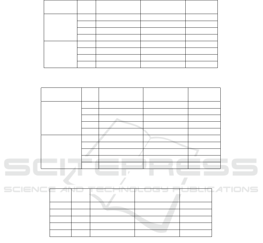
Table 2: Results obtained through the use of global appearance descriptors based on analytic methods (HOG and gist) to solve

visual localization.

Descriptor Size Error loc. (cm)

Time comp.

descriptor (ms)

Time pose

est. (ms)

HOG

64 16,34 ± 0, 78 44, 64 0,38

128 16,23 ± 0, 73 45, 27 0,51

256 16,22 ± 0, 69 45, 33 2,48

512 16,17 ± 0, 69 46, 52 4,75

gist

128 5,19 ± 0, 18 10,30 0,45

256 5,11 ± 0, 17 11,98 2,19

512 5,09 ± 0, 16 21,21 4,17

1024 5,08 ± 0, 16 40,07 10,72

Table 3: Results obtained through the use of global appearance descriptors based on auto-encoders (auto-enc-Frib and auto-

enc-SUN) to solve visual localization.

Descriptor Size Error loc. (cm)

Time comp.

descriptor (ms)

Time pose

est. (ms)

auto-enc-Frib

10 599,83 ± 3, 83 49,79 0,25

50 8,61 ± 2, 29 138,64 0,44

100 7,04 ± 0, 85 249,55 0,59

200 7,45 ± 0, 23 473,59 0,93

500 7,22 ± 0, 19 1166,49 4, 54

auto-enc-SUN

10 362,73 ± 22, 77 54,99 0,28

50 520,85 ± 29, 66 138, 61 0,43

100 916,16 ± 31, 58 252, 39 0,59

200 327,25 ± 21, 39 477, 48 0,90

500 5,31 ± 0, 34 1125,06 4, 66

Table 4: Results obtained through the use of global appearance descriptors based on places CNN (layers ’conv4’, ’conv5’,

’fc6’, ’fc7’ and ’fc8’) to solve visual localization.

Layer Size Error loc. (cm)

Time comp.

descriptor (ms)

Time pose

est. (ms)

conv4 169 5,03 ± 0, 02 6,64 1,62

conv5 169 5,09 ± 0, 17 6,66 0,63

fc6 4096 5,14 ± 0, 18 7,42 34,38

fc7 4096 16,71 ± 0, 84 8, 58 33, 22

fc8 205 24,22 ± 6, 44 8, 88 0, 72

namic dataset with panoramic images has been used

to evaluate the experiments. Five global appearance

descriptors have been evaluated: two based on an-

alytic methods (HOG and gist), two based on auto-

encoders and one based on CNN layers. The size of

each descriptor is varied through either tuning some

parameters (such as the number of bins in HOG or the

size of hidden representation of the auto-encoders) or

selecting a different layer in the CNN case. The lo-

calization error, the computing time to calculate the

descriptor and the computing time to estimate the po-

sition of the robot have been used as parameters to

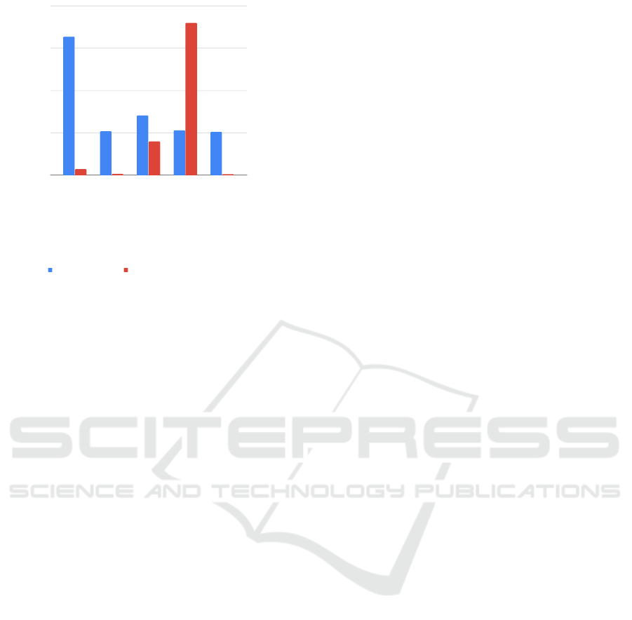
measure the efﬁciency of these descriptors. The ﬁg. 4

shows the results obtained for the best conﬁguration

of each descriptor evaluated. From that ﬁgure, we can

conclude that the minimum localization error is ob-

tained through the CNN-based descriptor option, but

the gist descriptor and the auto-enc-SUN descriptor

show results quite similar. The CNN-based descrip-

tor introduces also the best option regarding the com-

puting time to calculate the descriptor. Nevertheless,

regarding the time to estimate the pose of the robot,

HOG is the fastest.

Regarding the use of auto-encoders, using an auto-

encoder which has been trained with images that

belong to the environment outputs good-enough ac-

curacy results. The general auto-encoder proposed

through training a generic panoramic dataset works

acceptably in the case of high size of hidden represen-

tation, hence this leads to high computing times. Nev-

ertheless, its use as tool to obtain global appearance

descriptors for panoramic images would be valid and

An Evaluation between Global Appearance Descriptors based on Analytic Methods and Deep Learning Techniques for Localization in

Autonomous Mobile Robots

289

Descriptor

Error loc. (cm)

Time comp.descriptor (ms)

250

500

750

1000

1250

HOG

gist

auto-enc-Frib

auto-enc-SUN

CNN-conv5

Error loc. (cm) Time comp. descriptor (ms)

Figure 4: Summary of the best conﬁguration for each de-

scriptor studied.

the advantage of this method is that the auto-encoder

is trained just once, then the tool is suitable indepen-

dently the environment.

As for the use of CNN-based descriptors, we have

proved that the ﬁrst layers can output very interest-

ing descriptors despite these are not fully convolu-

tional layers (typically proposed to obtain descrip-

tors). Moreover, the descriptors related to the ’conv4’

and ’conv5’ layers have produced the optimal local-

ization solutions among all the methods evaluated:

size of descriptor relatively small (which leads to fast

times to estimate the position), low computing time

to calculate the descriptor and very accurate localiza-

tion (average error around 5 cm for a test dataset and a

training dataset whose average distance between im-

ages is around 4 cm and 20 cm respectively).

ACKNOWLEDGEMENTS

This work has been supported by the Generalitat Va-

lenciana through grant ACIF/2017/146 and by the

Spanish government through the project DPI 2016-

78361-R (AEI/FEDER, UE): “Creaci

on de mapas

mediante m

etodos de apariencia visual para la nave-

gaci

on de robots.”

REFERENCES

Cebollada, S., Pay

a, L., Mayol, W., and Reinoso, O. (2019).

Evaluation of clustering methods in compression of

topological models and visual place recognition us-

ing global appearance descriptors. Applied Sciences,

9(3):377.

Dalal, N. and Triggs, B. (2005). Histograms of oriented

gradients fot human detection. In In Proceedings of

the IEEE Conference on Computer Vision and Pattern

Recognition, San Diego, USA. Vol. II, pp. 886-893.

Gao, X. and Zhang, T. (2017). Unsupervised learning to de-

tect loops using deep neural networks for visual slam

system. Autonomous robots, 41(1):1–18.

Hubens, N. (2018). Deep inside: Autoencoders.

https://towardsdatascience.com/deep-inside-

autoencoders-7e41f319999f. Accessed February

11, 2019.

Korrapati, H. and Mezouar, Y. (2017). Multi-resolution

map building and loop closure with omnidirectional

images. Autonomous Robots, 41(4):967–987.

Leonardis, A. and Bischof, H. (2000). Robust recognition

using eigenimages. Computer Vision and Image Un-

derstanding, 78(1):99–118.

Mancini, M., Bul

o, S. R., Ricci, E., and Caputo, B. (2017).

Learning deep nbnn representations for robust place

categorization. IEEE Robotics and Automation Let-

ters, 2(3):1794–1801.

Naseer, T., Burgard, W., and Stachniss, C. (2018). Robust

visual localization across seasons. IEEE Transactions

on Robotics, 34(2):289–302.

Oliva, A. and Torralba, A. (2006). Building the gist of as-

cene: the role of global image features in recognition.

In Progress in Brain Reasearch: Special Issue on Vi-

sual Perception.Vol. 155.

Pay

a, L., Peidr

o, A., Amor

os, F., Valiente, D., and Reinoso,

O. (2018). Modeling environments hierarchically with

omnidirectional imaging and global-appearance de-

scriptors. Remote Sensing, 10(4):522.

Pronobis, A. and Caputo, B. (2009). COLD: COsy Lo-

calization Database. The International Journal of

Robotics Research (IJRR), 28(5):588–594.

Rom

an, V., Pay

a, L., and Reinoso, O. (2018). Evaluat-

ing the robustness of global appearance descriptors

in a visual localization task, under changing lighting

conditions. In ICINCO 2018. 15th International Con-

ference on Informatics in Control, Automation and

Robotics, Porto (Portugal), 29-31 July 2018, pages

258–265.

Su, Z., Zhou, X., Cheng, T., Zhang, H., Xu, B., and Chen,

W. (2017). Global localization of a mobile robot us-

ing lidar and visual features. In 2017 IEEE Interna-

tional Conference on Robotics and Biomimetics (RO-

BIO), pages 2377–2383.

Xiao, J., Ehinger, K. A., Oliva, A., and Torralba, A. (2012).

Recognizing scene viewpoint using panoramic place

representation. In Computer Vision and Pattern

Recognition (CVPR), IEEE Conference on, pages

2695–2702.

Xu, J., Xiang, L., Liu, Q., Gilmore, H., Wu, J., Tang,

J., and Madabhushi, A. (2016). Stacked sparse au-

toencoder (ssae) for nuclei detection on breast cancer

histopathology images. IEEE Transactions on Medi-

cal Imaging, 35(1):119–130.

Xu, S., Chou, W., and Dong, H. (2019). A robust indoor lo-

calization system integrating visual localization aided

ICINCO 2019 - 16th International Conference on Informatics in Control, Automation and Robotics

290

by cnn-based image retrieval with monte carlo local-

ization. Sensors, 19(2):249.

Zhou, B., Lapedriza, A., Xiao, J., Torralba, A., and Oliva,

A. (2014). Learning deep features for scene recog-

nition using places database. In Advances in Neural

Information Processing Systems, pages 487–495.

Zhou, X., Su, Z., Huang, D., Zhang, H., Cheng, T., and Wu,

J. (2018). Robust global localization by using global

visual features and range ﬁnders data. In 2018 IEEE

International Conference on Robotics and Biomimet-

ics (ROBIO), pages 218–223.

An Evaluation between Global Appearance Descriptors based on Analytic Methods and Deep Learning Techniques for Localization in

Autonomous Mobile Robots

291