Theoretical and Experimental Modal Analysis of a 6 PUS PKM
Francesco La Mura
1 a
, Hermes Giberti
1 b
, Linda Pirovano
2
and Marco Tarabini
2
1
Universita’ degli Studi di Pavia, Dipartimento di Ingegneria Industriale e dell’Informazione,
Via A.Ferrata 5, 27100 Pavia, Italy
2
Politecnico di Milano, Department of Mechanical Engineering, 20156 Milano, Italy
Keywords:
Modal Analysis, Parallel Kinematics Machines, Multibody, Natural Frequencies.
Abstract:
In this article the modal analysis of a manipulator is presented and discussed from a theoretical and experimen-
tal perspective. The work focuses on both the simulation and the experimental stages of the modal analysis on
six DOF parallel kinematics machine. In particular, the behavioural vibrational trend of the kinematics struc-
ture under analysis is presented within the entire workspace. Critical aspects of each test phase are highlighted
as well as data post processing methods used. Finally, a map capable of summarizing the modal analysis
results is shown.
1 INTRODUCTION
Differing poses of a manipulator within the
workspace can show completely different be-
haviour in terms of natural frequencies that could
cause serious vibrations and consequently instability
in the movement of the end effector, reducing accu-
racy (Mejri et al., 2016; Wiens and Hardage, 2006;
Silvestri et al., 2011; Confalonieri et al., 2018). This
aspect must be taken into consideration when one
is dealing with the design of a new robotic device
and in particular in the case of a parallel kinematic
architecture where the highly non linear kinematics
and the difficulty in realising joints and kinematic
constraints make the a priori evaluation of this
problem extremely difficult to assess.
In this work a procedure used for the modal char-
acterisation of a 6 DOF PKM for HIL testing is pre-
sented and analysed in depth. This device, called
Hexafloat, was designed and realised within the am-
bit of the H2020, LIFES50+ project at the Politecnico
di Milano (Bayati et al., 2014; Giberti et al., 2018).
By using this robot one can move a scaled model of
a wind turbine within the wind tunnel, simulating a
floating wind generator moving in a deep sea environ-
ment (Bayati et al., 2017; Giberti and Ferrari, 2015).
The Robot target position and orientation are cal-
culated in real-time resolving floater dynamics within
a force loop(La Mura et al., 2018b). This aspect
joined to the high inertia of the scaled wind turbine,
its flexibility and the required dynamics bandwidth of
a
https://orcid.org/0000-0001-5143-7120
b
https://orcid.org/0000-0001-8840-8497
the floater must be taken into account carefully in or-
der to obtain a good transparency behaviour (La Mura
et al., 2018a) of the HIL device. In order to obtain
these results, it is useful to identify the Hexafloat nat-
ural frequencies. This analysis can be limited to the
manipulator first natural frequency. The main goal is
to verify that the robot has its first natural frequency
well above both the range exploited by the floater mo-
tion (0 − 3hz), and the first frequencies of the turbine
being tested. For this type of study simulated and ex-
perimental analysis must be conducted together in or-
der to interpret the results correctly and support the
definition of the experimental setup.
Figure 1: Hexafloat robot main components.
276
Mura, F., Giberti, H., Pirovano, L. and Tarabini, M.
Theoretical and Experimental Modal Analysis of a 6 PUS PKM.
DOI: 10.5220/0007836902760283
In Proceedings of the 16th International Conference on Informatics in Control, Automation and Robotics (ICINCO 2019), pages 276-283
ISBN: 978-989-758-380-3
Copyright
c
 2019 by SCITEPRESS – Science and Technology Publications, Lda. All rights reserved

2 MULTIBODY MODEL
Hexafloat PKM architecture, shown in the figure 1 is
made up of three main components: a platform, car-
rying the turbine and load sensors; six identical legs
each belonging to a different kinematic chain; six ac-
tuation chains made up of a translating carriage, a
joint holder, a lead screw and a brushless motor di-
rectly connected to it.
The objectives of the analysis described in this pa-
per are, for all possible configurations of the robot
within its workspace to evaluate modal shapes and
their variation in different poses and to define the con-
figurations corresponding to absolute and local min-
ima of the first natural frequency.
In order to meet these objectives, the Hexafloat
model is developed with Adams
R

, a multibody soft-
ware able to reproduce robot dynamics and to perform
a vibration study, choosing between rigid and flexi-
ble behaviour among different components. There-
fore, few components have been neglected or simpli-
fied in order to reduce computational cost taking into
account major components influences.
The platform is modelled as a rigid body due to
its specifically designed shape, compact dimensions,
high performance materials that bring to orders of
magnitude lower deformations compared to the link
ones.
Links model are made of three flexible bodies: at
the far end of the link, two elements made of steel per-
fectly reproduce the geometry, dimensions and mass
parameters of the connecting rod, bearing case and
distance washer while in the middle an aluminium
hole cylinder stands for the main leg component. Slid-
ers are a simplification of joints located at the basis
and they replicate the behaviour of a translating mass.
Moreover, the robot model is completely
parametrized and created through the use of
Adams
R

MACRO.
This approach, combined with Co-Simulation be-
tween Matlab and Adams
R

, is able to efficiently ex-
plore all different configuration needed.
Stiffness, dumping and load transfer to actuators
change widely depending on the configuration as-
sumed. Natural frequencies evaluation is performed
investigating a grid of positions assumed by the Hex-
afloat TCP on three different planes fig. 2.
That are defined considering a rotation of an an-
gle φ around the z global axis. The angle φ cov-
ers three different values: 0
◦
,45
◦
and 90
◦
. The first
plane with φ = 0
◦
correspond to global Y-Z plane,
while the last one, φ = 90
◦
, identifies global X-Z
plane. On each plane discretization steps are defined,
of 25mm along Z and Y axes and 50mm along X-
Figure 2: Testing points for the simulation.
axis, as shown in fig. 2. The grid points are defined
in order to have always 7 points along each plane
axis, thus a total of 49 points in each plane. Lower
and upper bounds for both X, Y and Z are given by
nominal workspace dimensions of [±150, ±75,±75]
mm, around nominal Home Position (with null ori-
entation and position coordinates [0,0,463.6]). The
platform orientation is described by a set of three car-
danic angles, called roll, pitch and yaw (α,β,γ), re-
spectively as a rotation around X-axis, Y-axis and Z-
axis. With the following values: Roll α −5
◦
,0
◦
,5
◦
;
Pitch β: −8
◦
,−4
◦
,0
◦
,4
◦
,8
◦
and Yaw γ: −3
◦
,0
◦
,3
◦
.
The natural frequencies evaluation was performed
for all the possible combinations of these three angles
with an iterative procedure: for each position in the
grid, the Adams
R

MACRO routine is run and a new
model is created for every possible orientation. Given
45 different angular configurations for each point, a
total of 2205 combinations are tested on every plane.
In each point a static equilibrium is imposed and the
first eigenfrequency is evaluated.
3 SIMULATION RESULTS AND
DISCUSSION
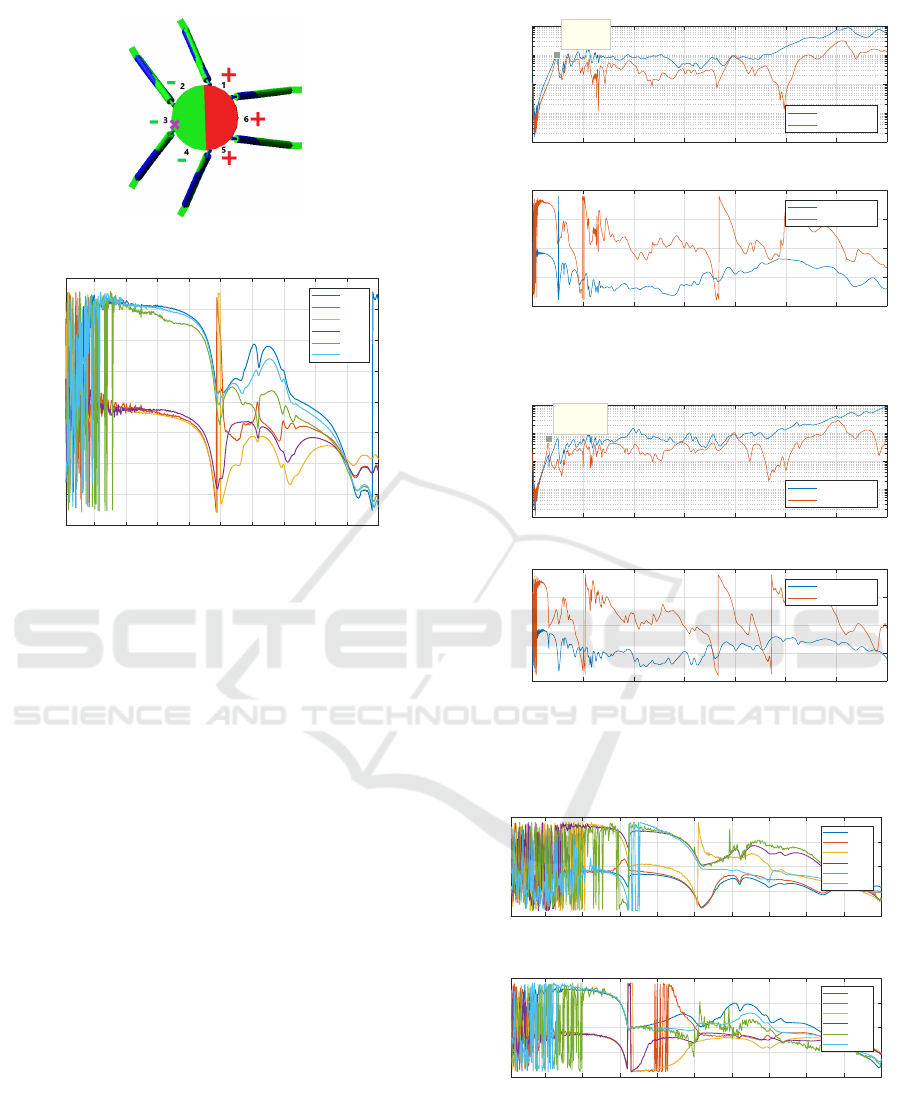
Trends results on φ = 0
◦
plane are shown in fig. 3.
Each coloured plane identifies a fixed orientation con-
figuration. The resulting surfaces show the variation
of the first frequency while moving inside the φ = 0
◦
plane, thus changing Y-Z value on the grid. The over-
all trend is most of the time a paraboloid, with a max-
imum value for DOF combination corresponding to
robot best and stiffest attitude. Frequency mean value,
standard deviation and percentage maximum varia-
tion are computed as well. All this statistical descrip-
tors are reported in tab. 1.
Theoretical and Experimental Modal Analysis of a 6 PUS PKM
277

(a) Frequency distribution for
different Roll angles
(b) Frequency distribution for
different Pitch angles
(c) Frequency distribution for
different Yaw angles
Figure 3: Frequency distributions on φ = 0
◦
plane (Y-Z).
Table 1: Results summary on the plane 0
◦
.
Angle Min[Hz] Max[Hz] Mean[Hz] Std[Hz] Max.∆f[%]
α
0
◦
143.67 171.25 161.71 6.79 16.11
5
◦
123.73 155.49 144.15 7.07 16.61
−5
◦
123.64 155.29 144.00 7.04 16.58
β
0
◦
143.67 171.25 161.71 6.79 16.11
4
◦
137.75 154.42 149.28 4.27 10.73
−4
◦
134.21 151.87 146.13 4.24 11.63
8
◦
122.28 134.35 129.69 3.42 8.98
−8
◦
116.26 129.87 124.29 4.00 10.39
γ
0
◦
143.67 171.25 161.71 6.78 16.11
3
◦
143.37 171.14 161.58 6.80 16.23
−3
◦
143.51 171.14 161.58 6.80 16.14
Roll Angle Influence: as shown in fig. 3a, for pos-
itive Roll rotations, maximum frequencies are regis-
tered along positive Y-axis direction while for nega-
tive rotations maxima are located along negative Y-
axis direction, showing a symmetric distribution as
expected. Z variation reveal an optimum height on
which first frequency have a local maximum and
whose value change with Y and angle combinations.
Absolute highest and lowest frequencies are regis-
tered at Y boundaries. Angular rotations of the same
sign of the Y displacement lessen the machine asym-
metry and so the manipulator assumes a more struc-
turally rigid position, thus enhancing 1st natural fre-
quency value.
Pitch Angle Influence: by varying the Pitch angle,
frequency distribution exhibits changes as well. The
same trend is preserved for every angle value, except
for mean value that decreases as the angle increases
its magnitude. This behaviour is clearly shown in
fig. 3b. The lowest frequencies are registered for
β = −8
◦
for which Hexafloat legs are in the most
asymmetric configuration. Negative rotations induces
always a larger frequency reduction with respect to
positive rotation of the same magnitude, this is due to
different number of legs approaching singular config-
uration. Greater influence of Pitch angle is near the
centre of the Y-Z plane while at the boundaries, the
frequency decreases due to the already high asymme-
try of the legs arrangement caused by Y and Z varia-
tion.
Yaw Angle Influence: the frequency distribution is
not affected by a variation of Yaw angle as shown in
fig. 3c, as only differences caused by non zero Y and
Z coordinates arise.
The same analysis was performed for φ = 90
◦
and
φ = 45
◦
. For the sake of brevity the results are not
reported.
4 EXPERIMENTAL MODAL
ANALYSIS
Experimental modal analysis is based on the measure-
ments of structure FRFs. This measurement requires
an excitation in one or more locations and collec-
tion of vibratory response in multiple positions (Fu
and He, 2001). In many experimental investigation
regarding manipulators natural frequencies (Palmieri
ICINCO 2019 - 16th International Conference on Informatics in Control, Automation and Robotics
278

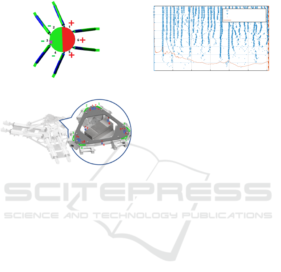
Figure 4: First vibration mode: vertical displacement sign
of the tilting platform.
Figure 5: Accelerometers location (blue), measuring direc-
tion (red) and hitting points (green).
et al., 2014; Vu et al., 2016), the entire structure is
scanned by placing sensors onto each structural ele-
ment.
By means of the modal shapes tracking obtained
by the simulation, sensors number and placement
was chosen effectively, avoiding uselessly expensive
and burdensome setup and data post processing. As
shown in fig.4, being the first and second mode char-
acterised by a clear platform tilt, namely a rigid rota-
tion, each platform point not located on the rotation
axis, have an acceleration component in Z direction.
The rotation axis virtually cut the platform in two sec-
tion, each of which has homogeneous Z acceleration
sign (fig.4). Analysing the reciprocal phase between
accelerometers and input force, modal shapes can be
then re-identified from experimental data.
Six accelerometers are located onto the platform:
one placed onto each joint block and the other three
arranged on the platform in between of each legs cou-
ple. The described arrangement allows to have at
least 2 sensors detecting one of the two coupled fre-
quencies. For a robust mode identification, also ac-
celerometers not measuring along Z direction are re-
quired. Three more sensors are positioned onto the
platform (7,8 and 9 in fig. 5), each one onto a joint
block, measuring in the direction tangent to the circle
enclosing the platform joints.
0.1 0.2 0.3 0.4 0.5 0.6
Frequency (kHz)
0
10
20
30
40
50
60
70
80
Model Order
10
-16
10
-14
10
-12
10
-10
10
-8
10
-6
10
-4
10
-2
Magnitude
Stabilization Diagram
Stable in frequency
Stable in frequency and damping
Not stable in frequency
Averaged response function
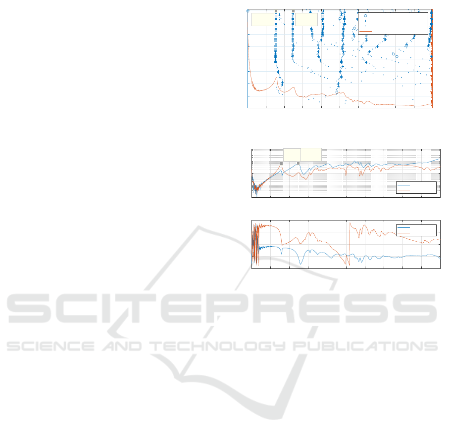
Figure 6: Stability diagram obtained with multiple LSCE
analysis.
4.1 Experimental Procedure
The procedure adopted during the experimental tests
is briefly summarized as follows. Hexafloat is moved
in the i-th testing pose. The impact hammer hits the
structure in the first hitting location for the i-th pose
and the response is acquired for at least 5s. This op-
eration is repeated 5 times. The impact hammer hits
the structure in the second hitting location for the i-th
pose and the response is acquired for at least 5s. This
operation is repeated 5 times. Orientation is changed
and points 2 and 3 are repeated until all possible an-
gle combination are covered. After that, point 1 is re-
peated and another grid point on the plane is explored.
This procedure is repeated on each chosen plane. Im-
pact points are chosen by observing simulated modal
shapes changing detected and avoiding vibratory nods
while maximizing expected vertical acceleration lec-
ture.
4.2 Measurements Setup
Measurement chain components are briefly summa-
rized hereafter. Impact hammer: PCB
R

086C03
model with a 2.25mV/N sensitivity. The hammer is
equipped with a medium hardness plastic tip and a
extender mass weight of 75grams with the aim of in-
troducing a suitable amount of energy able to excite
the structure over a wide frequency range. Piezoelec-
tric accelerometers: Bruel&Kjaer
R

4508 model has
high sensitivity, low mass and small physical dimen-
sions that make this sensor suitable for modal investi-
gation in rough environments. They have a frequency
range of 0.4–6000Hz, a 10 mV/ms
−2
sensitivity and
a mass of 4.8grams. DAQ system: NI
R

Compact-
DAQ-9178 with 8 slots in which C-Series I/O module
are plugged in. Three NI
R

9402 C-series I/O mod-
ule equipped with 4 bidirectional channels with BNC
connectivity and a 55ns update rate are employed.
Signals are acquired by mean of Politecnico di Milano
Theoretical and Experimental Modal Analysis of a 6 PUS PKM
279

MeasLab software. The signals are acquired with a
sampling rate of 2048 Hz and each test has a duration
of 5s, thus ensuring a frequency resolution of 0.2Hz.
5 DATA POST-PROCESSING
METHODS
Natural frequencies extrapolation from system Fre-
quency Response Functions (FRFs) is a key step
in data post-processing. This operation is done by
checking FRFs plot and using other methods such
as Least-Square-Complex-Exponential (LSCE). This
method requires the computation on impulse response
function associated to each FRF. Each impulse re-
sponse is expressed by a series of complex damped
sinusoids, in the form of exponential functions, which
contain eigenvalues and eigenvectors (Brandt, 2011;
Allemang et al., 1994).
The LSCE method allows one to individuate the
system natural frequencies through system poles ex-
traction. The number of poles considered in the
analysis is really affecting the obtained results. To
overcome this limitation, the identification is carried
out for increasing model orders. As the model or-
der is increased, more and more modal frequencies
are estimated but the estimates of the physical modal
parameters will stabilize as the correct model order
is found (Allemang et al., 1994). Physical modes
are easily distinguish from spurious modes related to
noise or other computational issue: the first ones con-
stantly arise for different model order while the sec-
ond ones randomly appears. A straightforward exam-
ple is reported in fig. 6. The vertical straight lines
in fig. 6 show up in correspondence of natural fre-
quencies, but only the ones characterised by verti-
cal lines both stable in frequency and damping can
be trusted. The natural frequency extraction is done
for all the measured data in all the tested Hexafloat
poses by mean of the natural frequencies evaluation
from stability diagram of the averaged FRFs mea-
sured in each pose. The doubly stable obtained values
are compared with the ones in FRFs magnitude and
phase plots to confirm the results. Figure 7 demon-
strates the goodness of both results obtained with sta-
bility diagram and the ones reported in FRF plot for
the
{
−150,0,538.6, 0
◦
,−8
◦
,0
◦
}
configuration. Use-
ful methods adopted for coupled modes are Single
Value Decomposition(SVD) and Complex Mode Indi-
cator Function(CMIF), not described here for brevity.
0.02 0.04 0.06 0.08 0.1 0.12 0.14 0.16 0.18 0.2
Frequency (kHz)
0
10
20
30
40
50
60
70
80
Model Order
10
-14
10
-12
10
-10
10
-8
10
-6
10
-4
10
-2
Magnitude
Stabilization Diagram
Stable in frequency
Stable in frequency and damping
Not stable in frequency
Averaged response function
X: 0.03102
Y: 79
X: 0.04947
Y: 79
(a) Stability diagram
0 20 40 60 80 100 120 140 160 180 200
Frequency (Hz)
10
-4
10
-2
10
0
Magnitude [m/s
-2
]
hit location #2
hit location #4
0 20 40 60 80 100 120 140 160 180 200
Frequency (Hz)
-200
-100
0
100
200
Phase [°]
hit location #2
hit location #4
X: 31.6
Y: 0.06227
X: 49.6
Y: 0.0638
(b) Acelerometer #1 FRF
Figure 7: 1st and 2nd natural frequencies in
{
−150,0,538.6,0
◦
,−8
◦
,0
◦
}
configuration.
6 EXPERIMENTAL RESULTS
Due to the mathematical model approximation, the
1st natural frequencies is lower compare to the sim-
ulated one: taking into consideration the Home Posi-
tion configuration with null angular orientation, 47 Hz
is the experimental value compared to 170 Hz the one
simulated. This difference is due to model approxi-
mations, such as passive joints considered ideal and
rigid, as well as the fixed base.
Despite this difference and according to the ob-
jectives of the work, simulations and experimental
results succeed in minimum frequency configuration
identification, first mode trends evaluation and mode
shapes re-construction.
The first resonance peak is at a very low frequency
and it exhibits a clear 180
◦
phase change, thus reveal-
ing the presence of a physical mode of vibration. This
resonance peak shows up in all accelerometers FRFs
at almost the same frequency value in both two hit-
ting points. An example is provided in fig. 8, in which
the platform is hit in location #4, indicated with violet
cross, while numbers identify sensors location. Look-
ing at the sign of the phase diagram (fig. 8b), the plat-
ICINCO 2019 - 16th International Conference on Informatics in Control, Automation and Robotics
280

(a) Vibration mode signs
10 20 30 40 50 60 70 80 90 100
Frequency [Hz]
-200
-150
-100
-50
0
50
100
150
200
Phase [°]
acc. 1
acc. 2
acc. 3
acc. 4
acc. 5
acc. 6
(b) Phase plot
Figure 8: Vibration sign check.
form exhibits a vibration similar to the one resulting
from simulation: half of the platform vibrate in phase
with the hammer hit while the other one in counter
phase
Additional peaks appear at a frequency around
60Hz. This multiple peaks does not correspond to
a clear phase shift, thus revealing the possibility of
being induced by few other symmetric components
that does not mainly vibrate in the investigate direc-
tion. A prominent peak characterised by a clear phase
shift emerges around 80 Hz. Analysing in detail the
sign of the phase plot for all the accelerometers, it
can be stated the vibration is always in phase with
the hit direction, thus highlighting a prominent move-
ment along z-direction with no relevant rotation and
so discarding this one from the simulated 1st mode of
vibration search.
Verification of mode decoupling is also required.
The FRFs computed from different hits should be
characterised by not all the accelerometers reading
the same first frequency value, being some of them
in nodes for one of the two no more coupled modes.
The above mentioned requirements can be found in
fig. 7b and 9. For the sake of brevity, only the
{
−150,0,538.6, 0
◦
,−8
◦
,0
◦
}
pose configuration is re-
ported even though the correct simulated behaviour is
found for all the experimentally tested poses. From
0 100 200 300 400 500 600 700
Frequency (Hz)
10
-4
10
-2
10
0
Magnitude [m/s
-2
]
hit location #2
hit location #4
0 100 200 300 400 500 600 700
Frequency (Hz)
-200
-100
0
100
200
Phase [°]
hit location #2
hit location #4
X: 47.4
Y: 0.1025
(a) Home position
0 100 200 300 400 500 600 700
Frequency (Hz)
10
-4
10
-2
10
0
Magnitude [m/s
-2
]
hit location #2
hit location #4
0 100 200 300 400 500 600 700
Frequency (Hz)
-200
-100
0
100
200
Phase [°]
hit location #2
hit location #4
X: 31.6
Y: 0.06227
(b)
{
−150,0,538.6,0
◦
,−8
◦
,0
◦
}
configuration
Figure 9: Accelerometer #1 FRF.
10 20 30 40 50 60 70 80 90 100
Frequency [Hz]
-200
-100
0
100
200
Phase [°]
acc. 1
acc. 2
acc. 3
acc. 4
acc. 5
acc. 6
(a) hammer hit #2
10 20 30 40 50 60 70 80 90 100
Frequency [Hz]
-200
-100
0
100
200
Phase [°]
acc. 1
acc. 2
acc. 3
acc. 4
acc. 5
acc. 6
(b) hammer hit #4
Figure 10: Phase diagram of FRF in
{
−150,0,538.6,0
◦
,−8
◦
,0
◦
}
configuration, zoom on
[0:100]hz.
47Hz in Home Position, peak value moves to 31Hz,
accordingly with simulated reduction (98 Hz vs. the
Theoretical and Experimental Modal Analysis of a 6 PUS PKM
281

Home Position 170 Hz). A new peak appear at 49 Hz,
not present in the Home Position, validating the de-
coupling of the two modes due to the asymmetry of
the manipulator structure in this pose (fig. 7b).
Once correspondence between experimentally
identified modes and simulated one has been as-
sessed, it is possible to compare frequency shift
trends. Since absolute frequency values do not cor-
respond, the comparison is done normalizing all the
frequency values with respect to results in maximum
Z and null X, Y. Instead, when examining angle vari-
ation influence, a different normalization is adopted:
data are normalized with respect to the null angle con-
figuration, referring to the value associated to x = 0 in
90
◦
plane or y = 0 in 0
◦
plane.
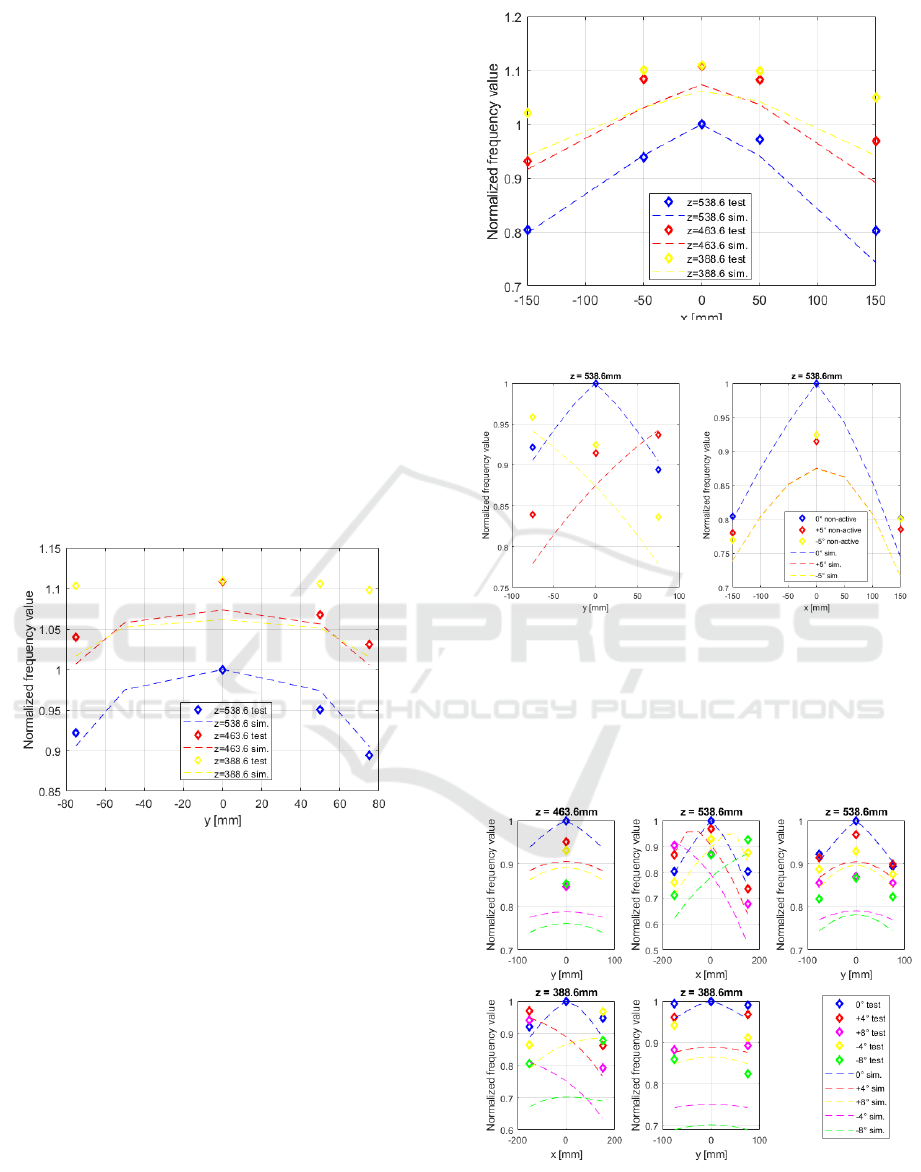
Translation Effect on Y-Z Plane: the frequency dis-
tribution in 0
◦
plane has the expected parabolic trend
(fig. 11). Experimental data confirm the symmetric
data distribution obtained in simulations. The be-
haviour of normalized data as z-coordinate decreases
is confirmed as an increase in frequency is correctly
detected.
Figure 11: 0
◦
plane frequency trend.
Translation Effect on X-Z Plane: both simulated
and experimental frequency trends on 90
◦
plane for
different z values are characterised by a parabolic
shape (fig. 12). Z-coordinate effect appears stronger
on experimental results at workspace boundary re-
gions.
Roll Influence on X-Z Plane: a good correspon-
dence in terms of frequency trend can be extrapolate
from X-Z plane (fig 13), in which the parabolic dis-
tribution shows up for both experimental and simu-
lated results. As expected, positive and negative Roll
angles does not causes a significant frequency differ-
ence. Experimental results shown higher normalized
frequencies compared to the normalized simulated re-
sults, thus revealing slightly less sensibility to pose
change.
Pitch Influence on Y-Z Plane: fig. 14 illustrates
Figure 12: 90
◦
plane frequency trend.
Figure 13: Roll angle influence.
frequency distribution caused by Pitch angles. Nor-
malized frequency values obtained from experiments
are greater with respect to the ones computed in
Adams
R

. Anyhow the distribution trend is correctly
reproduced.
Figure 14: Pitch angle influence.
Yaw Influence: as expected from the simulation,
experimental Yaw angle variations can be consid-
ICINCO 2019 - 16th International Conference on Informatics in Control, Automation and Robotics
282

ered negligible in the frequencies distribution into
workspace (fig. 15).
Figure 15: Yaw angle influence.
7 CONCLUSIONS
In this article, a complete methodology for modal
analysis of a 6 DOF parallel kinematics robot is
proposed. In alternative to literature methods, the
proposed procedure do not use complex simulations
setup and expensive experimental campaigns. Simu-
lation analysis has been designed in order to be simple
and effective, with the only support of a approximate
flexible-multibody model. Simulation campaign has
highlighted: modal shapes and their change through
workspace exploration, sensor and hitting points op-
timum configuration and minimum first frequency
robot configuration. These information has been used
for optimal experimental campaign design and iden-
tification of a small set of configuration on which
fine FEM simulation could be set up. Experimental
campaign has been setup with minimum amount of
sensors and effective testing procedure. A complete
data post processing method has been also proposed,
particularly suitable con complex PKM with coupled
modes and taking into account real world data issues.
REFERENCES
Allemang, R. J., Brown, D. L., and Fladung, W. (1994).
Modal parameter estimation: a unified matrix polyno-
mial approach. In Proceedings - SPIE The Interna-
tion Society For Optical Engineering, pages 501–501.
SPIE Internation Society For Optical.
Bayati, I., Belloli, M., Bernini, L., Giberti, H., and Zasso,
A. (2017). Scale model technology for floating off-
shore wind turbines. IET Renewable Power Genera-
tion, 11(9):1120–1126.
Bayati, I., Belloli, M., Ferrari, D., Fossati, F., and Giberti,
H. (2014). Design of a 6-dof robotic platform for wind
tunnel tests of floating wind turbines. Energy Proce-
dia, 53:313–323.
Brandt, A. (2011). Noise and vibration analysis: signal
analysis and experimental procedures. John Wiley &
Sons.
Confalonieri, M., Ferrario, A., and Silvestri, M. (2018).
Calibration of an on-board positioning correction sys-
tem for micro-edm machines. In EUSPEN Conference
Proceedings - 18th International Conference and Ex-
hibition, pages 153–154.
Fu, Z.-F. and He, J. (2001). Modal analysis. Elsevier.
Giberti, H. and Ferrari, D. (2015). A novel hardware-in-
the-loop device for floating offshore wind turbines
and sailing boats. Mechanism and Machine Theory ,
85(Supplement C):82 – 105.
Giberti, H., La Mura, F., Resmini, G., and Parmeggiani, M.
(2018). Fully mechatronical design of an hil system
for floating devices. Robotics, 7(3):39.
La Mura, F., Roman
´
o, P., Fiore, E., and Giberti, H. (2018a).
Workspace limiting strategy for 6 dof force controlled
pkms manipulating high inertia objects. Robotics,
7(1):10.
La Mura, F., Todeschini, G., and Giberti, H. (2018b).
High performance motion-planner architecture for
hardware-in-the-loop system based on position-based-
admittance-control. Robotics, 7(1):8.
Mejri, S., Gagnol, V., Le, T.-P., Sabourin, L., Ray, P., and
Paultre, P. (2016). Dynamic characterization of ma-
chining robot and stability analysis. The Interna-
tional Journal of Advanced Manufacturing Technol-
ogy, 82(1-4):351–359.
Palmieri, G., Martarelli, M., Palpacelli, M., and Carbonari,
L. (2014). Configuration-dependent modal analysis of
a cartesian parallel kinematics manipulator: numeri-
cal modeling and experimental validation. Meccanica,
49(4):961–972.
Silvestri, M., Pedrazzoli, P., Bo
¨
er, C., and Rovere, D.
(2011). Compensating high precision positioning ma-
chine tools by a self learning capable controller. In
Proceedings of the 11th international conference of
the european society for precision engineering and
nanotechnology, pages 121–124.
Vu, V.-H., Liu, Z., Thomas, M., Li, W., and Hazel, B.
(2016). Output-only identification of modal shape
coupling in a flexible robot by vector autoregressive
modeling. Mechanism and Machine Theory, 97:141–
154.
Wiens, G. J. and Hardage, D. S. (2006). Structural dy-
namics and system identification of parallel kinematic
machines. In ASME 2006 International Design En-
gineering Technical Conferences and Computers and
Information in Engineering Conference, pages 749–
758. American Society of Mechanical Engineers.
Theoretical and Experimental Modal Analysis of a 6 PUS PKM
283