Numerical Modelling of the Circulation and Pollution Transport

from Rivers and Wastewater Treatment Plants in the Sochi Coastal

Area

Nikolay Diansky

1,2,3

, Vladimir Fomin

, Irina Panasenkova

and Evgeniya Korshenko

Department of Numerical Modelling of Hydrophysical processes, Zubov State Oceanographic Institute, Moscow, Russia

Faculty of Physics, M.V. Lomonosov Moscow State University, Moscow, Russia

Institute of Numerical Mathematics, Russian Academy of Sciences, Moscow, Russia

Keywords: Black Sea, Coastal Circulation, Downwelling, Sea Ventilation.

Abstract: This paper provides a brief description of the technique for simulation Black Sea circulation and pollution

spreading in the Sochi coastal area. Two versions of the ocean circulation INMOM model are used: M1 model

with coarse spatial resolution of 4 km and M2 model with non-uniform spatial resolution. Large-scale

structure and mesoscale large eddies of Black Sea are simulated using M1 model. M2 model is applied for

simulating mesoscale and sub-mesoscale dynamics, in addition to simulating large-scale structure of the Black

Sea circulation in the coastal zone near Sochi. In this study we analyse the structure of horizontal and vertical

coastal currents and estimate concentration and spread of pollution. The results of numerical modelling in the

coastal zone were successfully validated using laboratory and observation data from Elkin et al., 2017.

1 INTRODUCTION

Numerical modelling of the dynamics of coastal

currents is a challenging, yet timely problem. Coastal

currents, in turn, define the dynamics of pollution

spreading.

This paper presents a technique for reproducing

circulation of the Black Sea and modelling the

spreading of pollutants in the Black Sea coastal zone

near Sochi. Three-dimensional sigma-coordinate

model of ocean circulation INMOM (Institute of

Numerical Mathematics Ocean Model) is used for

simulating the Black and Azov Seas’ dynamics. The

INMOM model is based on primitive equations of

ocean dynamics with incompressibility, hydrostatic

and Boussinesq approximations (Diansky, 2013).

The main objectives of this work are to study the

mechanism of vertical circulation and pollution

transport characteristics in the Sochi coastal area and

to validate the model by comparing the results of

https://orcid.org/0000-0002-6785-1956

https://orcid.org/0000-0001-8857-1518

https://orcid.org/0000-0002-8338-4825

https://orcid.org/0000-0003-2310-9730

numerical modelling to available laboratory

experiments and observations.

Small-scale coastal processes and their impact on

pollution spreading in the Big Sochi region in the

Black Sea has already been reviewed in the work by

Diansky et al., 2013. However, the results of

numerical modelling of pollutants’ vertical transport

were considered controversial, till laboratory

experiments studying downwelling coastal current

dynamics were carried out at the Shirshov Institute of

Oceanology, Russian Academy of Sciences (IO RAS)

(Elkin et al., 2017).

2 METHODOLOGY

Two versions of the INMOM model (model M1 and

model M2) were developed for simulation of

hydrophysical fields of the Black Sea.

378

Diansky, N., Fomin, V., Panasenkova, I. and Korshenko, E.

Numerical Modelling of the Circulation and Pollution Transport from Rivers and Wastewater Treatment Plants in the Sochi Coastal Area.

DOI: 10.5220/0007836203780383

In Proceedings of the 5th International Conference on Geographical Information Systems Theory, Applications and Management (GISTAM 2019), pages 378-383

ISBN: 978-989-758-371-1

2.1 The M1 Model for Simulation of

the Black and Azov Seas’

Circulation

The detailed description of the M1 model is provided

in the work by Diansky et al., 2013.

Computational grid covers the entire areas of the

Black and Azov Seas in the M1 model. It has uniform

horizontal resolution of 4 km and contains 287 × 160

nodes in the horizontal plane. The M1 time step

equals 5 minutes. It has forty nonuniformly

distributed vertical sigma levels.

Bathymetry data of the Black Sea were obtained

from the global GEBCO atlas with spatial resolution

of 30’’ available to download from www.gebco.net.

Three dimensional monthly mean climatic fields

of temperature and salinity for the Black Sea basin

made by the Marine Hydrophysical Institute of the

National Academy of Sciences of Ukraine (MHI

NASU) (Ivanov and Belokopytov, 2011) were used

as the M1 model initial conditions, after they were

interpolated on the M1 model grid.

Temperature and salinity horizontal turbulent

diffusion were parameterized using a second order

operator with coefficient of 50 m

–1

. Parametrization

of the horizontal viscosity was performed by an

operator of the fourth order with coefficient of 10

/s. Vertical turbulent processes were parameterized

according to Philander–Pacanovsky suggestions

(Pacanovsky and Philander, 1981): the coefficient of

vertical viscosity ranged from 10

–4

to 10

–3

/s, the

coefficient of vertical temperature diffusion varied in

the range from 0.5 × 10

–5

to 0.5 × 10

–4

/s and the

coefficient of vertical salinity diffusion ranged from

0.1 × 10

–5

to 0.1 × 10

–4

/s.

Condition of temperature and salinity zero fluxes

were set at the bottom and lateral boundaries. The

zero-velocity condition was set at the boundaries. The

free-slip condition was specified at the lateral

boundaries. Finally, squared friction was used at the

bottom.

The nudging condition was used for salinity with

the relaxation parameter of 1/120 day

–1

. This was

made to fit the model salinity to the climatic values at

the depths below 300 m. For surface salinity special

correction of its climatological values was added to

the salinity flux with the relaxation parameter

equaling 10 m/120 days. This coefficient means the

relaxation of the average over 10 m depth model

salinity to the climatic values with a 120 days time

step.

The atmospheric data consist of temperature and

humidity, wind speed at a height of 10 m, sea level

pressure, precipitation, and downwelling long- and

short-wave radiation. These atmospheric

characteristics were downloaded from the Era Interim

global atmospheric reanalysis of the European Center

for Medium Range Weather Forecast (ECMWF)

(https://apps.ecmwf.int/datasets/data/interim-full-

daily/levtype=sfc/). Bulk-formulas were used to

calculate sensible and latent heat fluxes, short- and

long-wave radiation, momentum flux and net salt

flux, consisting of evaporation, precipitation and

climatological runoff.

To set rivers’ discharge in the M1 model data

from the climatic year CORE (Coordinated Ocean-ice

Reference Experiments) (Large and Yeager, 2004)

was taken in the form of pseudoprecipitation

concentrated in the basins near the river mouths.

2.2 The M2 Model for Simulation of

the Black Sea Circulation and

Pollution Spreading

The M2 model was described in detail in Diansky et

al., 2013. Only the basic features will be mentioned

here.

M2 version of the INMOM model was applied to

simulate the Black Sea circulation with increased

resolution in the area of waters near the Sochi coast.

Spherical coordinates are used for writing primitive

model equations with one of the poles situated in the

land point with geographic coordinates (40.0052° E,

43.5913° N) near Krasnaya Skala village. Such grid

with variable step and refinement in the area of

interest makes it possible to vary horizontal resolution

from 50 m near Sochi to 5-9 km in the western part of

the Black Sea (Figure 1). The M2 model has twenty

nonuniformly distributed vertical sigma levels.

The M2 model computational grid has 759x600

nodes in the horizontal plane. In other words, the M2

grid is much larger than the M1 grid. The M2 model

time step is 30 s. Considering large domain dimension

and small time step the M2 model requires significant

computational resources and it is very time

consuming, in contrast to the M1 model, which has a

reasonable experiment time.

Vertical diffusion coefficients used in the

Philander–Pacanovsky parametrization were set to

the same values as in the M1 model. Horizontal

diffusion coefficients for temperature and salinity

were considered proportional to the spatial step of the

M2 model grid. Horizontal viscosity coefficient of the

forth order was set proportional to the square of the

spatial grid step.

Bottom bathymetry was defined similarly to the

M1 model, by interpolating global GEBCO data on

the M2 grid domain (Figure 2). Main rivers of the

Numerical Modelling of the Circulation and Pollution Transport from Rivers and Wastewater Treatment Plants in the Sochi Coastal Area

379

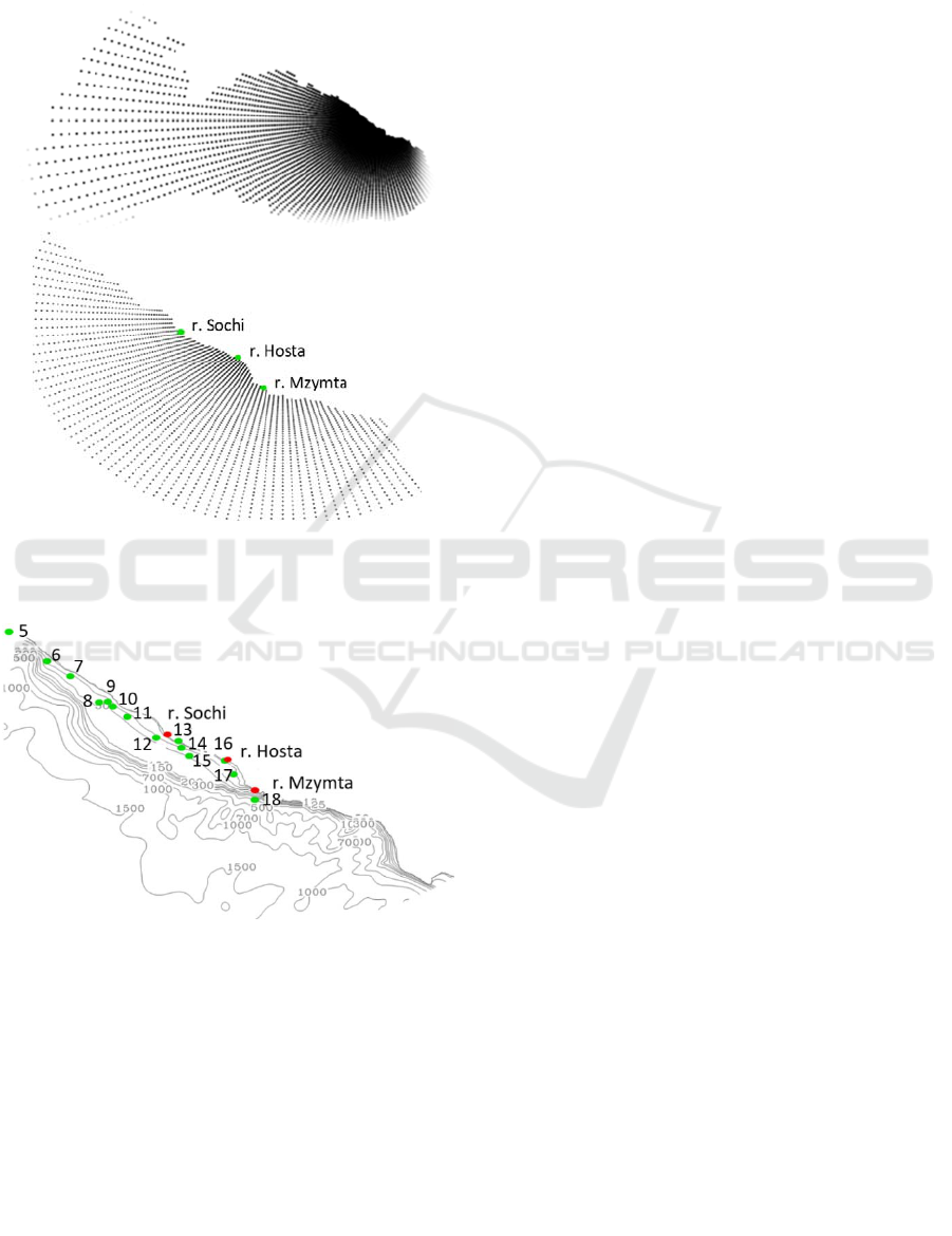
Sochi region (Sochi, Khosta, Mzymta) and 18 sewage

discharge pipe heads included into the model

experiment are marked on the Figure 2.

Figure 1: The M2 model computational grid with zooming

of the Big Sochi domain area with high resolution. Every

fifth point along each coordinate is showed.

Figure 2: Bottom bathymetry of the M2 model. Colored

points correspond to the rivers (red) and sewage discharge

pipe heads (green).

Both models are eddy-permitting ocean

circulation models which reproduce circulation of the

Black Sea. The Black Sea Rim Current, eddies which

accompany it, anticyclonic eddy vortices with

diameters up to 50–100 km are reproduced by M1

model with coarse resolution of 4 km. However, M2

model with high spatial resolution allows us to

simulate eddy circulation more qualitatively and

small-scale coastal processes in the area of interest (in

the eastern part of the Black Sea near Sochi).

Moreover, mesoscale and sub-mesoscale eddies have

a significant impact on the coastal water dynamics,

which, for their part, determine pollution spreading.

2.3 A Technique for Modelling the

Spread of Pollutants

A technique of numerical modelling of pollution

spreading was proposed using the M1 and M2

models. At first, the M1 model is used to calculate

Black and Azov Seas’ circulation for the specified

time period. Then, the M2 model is used to simulate

the Black Sea dynamics and calculate pollution

concentration and transport during the simulation

time of the pollution spreading. Initial conditions for

the M2 simulation start time is calculated by the M1

version of the model.

Equation of passive tracer transport–diffusion is

solved to estimate pollution characteristics in the M2

model. This equation is similar to the diffusion

equations used for temperature and salinity

calculation, except the fact that the monotonous

scheme of transport–diffusion is used and the

diffusion coefficient for a passive tracer provides

nonnegativity of the solution.

3 RESULTS AND DISCUSSION

Available laboratory and observation data along with

the results of the model simulation will be used to

study coastal circulation structure and pollution

spreading in the shelf slope zone of the Black Sea.

If coastal sea current reaches the bottom, bottom

Ekman layer is formed. In this layer in the Northern

Hemisphere the net water transport is 90 degrees to

the left of the surface current direction. In case if

cyclonic current flows along the sea eastern coast,

water in the bottom Ekman layer will be transported

from the coast, resulting in the downwelling current

accompanied by surface water sinking along an

inclined bottom.

In the eastern part of the Black Sea alongshore

current, as a part of large-scale cyclonic Rim Current,

leads to the formation of the downwelling coastal

current. Downwelling plays an important role in the

ventilation of stratified water masses. As a result of

enhanced ventilation, oxygen-rich surface waters

enter deeper layers of the Black Sea. In the work by

Elkin et al. (2017) it was suggested that this process

leads to oxygen ventilation of the Black Sea aerobic

layer. Furthermore, oxygen reduction in the coastal

ONM-CozD 2019 - Special Session on Observations and Numerical Modeling of the Coastal Ocean Zone Dynamics

380

zone has unfavorable influence on the ocean

biogeochemical cycles and marine ecosystems.

Sinking waters on the continental slope are one of

the poorly studied ventilation mechanisms for the

stably-stratified sea waters. Numerical modelling and

laboratory experiments are the basic methods of

studying this topic.

3.1 Numerical Experiment

We simulated pollution spreading during the flood

period from April 1, 2007 to April 30, 2007 using the

M2 model. The results of the Black Sea circulation

modelling from the M1 model on April 1, 2007 was

used as the initial conditions for the M2 model

running. The atmospheric forcing for the M2 model

was the same as for the M1 model.

In the numerical experiment the Sochi, Khosta,

and Mzymta rivers and 18 deepwater sewage pipes

were considered to be the main sources of pollutants

in the coastal waters of the Sochi region. The Data

about pipes’ locations and their discharges were

provided by the Sochi Special Center on

Hydrometeorology and Monitoring of the Black and

Azov Seas (SSCHM BAS).

As for the M1 model, the CORE database (Large

and Yeager, 2004) was used to get the river runoff

data, but for the discharges of the Mzymta, Sochi, and

Khosta rivers. These rivers’ discharges were

estimated using the real climatic discharges from the

work by Dzhaoshvili (1999). For the Sochi River

discharge equaled to 42 m

/s, for the Khosta River –

17 m

/s, and for the Mzymta River – 144 m

/s.

The coefficient of volume concentration of

conventional pollutant in the river waters was 0.03

according to the estimates of the Zubov State

Oceanographic Institute. The sewage waters from the

pipes were assumed to be completely polluted with

coefficient equaling 1.0 m

The technique for calculating concentration of the

pollutants in the cells of the grid domain was

discussed in Diansky et al. (2013). It was considered

that at each model time step the inflow of pollutants

in the grid cell was calculated in accordance with the

volume concentration coefficients of rivers and pipes

multiplied by the corresponding concentration and

the instantaneous dilution of pollutants over the grid

cell volume. Pollution total transport from rivers was

approximately 6 m

/s, and the total transport of

pollutants from all pipes was approximately 2 m

/s.

The pollution concentration was dimensionless

with the minimum considered level equaled to 10

–7

volume parts of pollutants in the water. This value

was comparable to the threshold limit value (TLV)

for the main pollutants in seawater (Diansky et al.,

2013).

Coastal currents play crucial role in the spread of

pollutants from the rivers and pipes. Since mesoscale

and sub-mesoscale eddies take the main part in

transportation of pollutants, if the model is eddy-

permitting, the accuracy of the model performance is

higher. The pattern of pollution distribution can show

involved eddy structures of the coastal currents in the

Black Sea. It was shown by Diansky et al. that the M2

model qualitatively reproduces horizontal dynamics:

the large-scale circulation (the Black Sea Rim

current) and the large quasi-geostrophic eddies of

≈20–100 km (mesoscale processes).

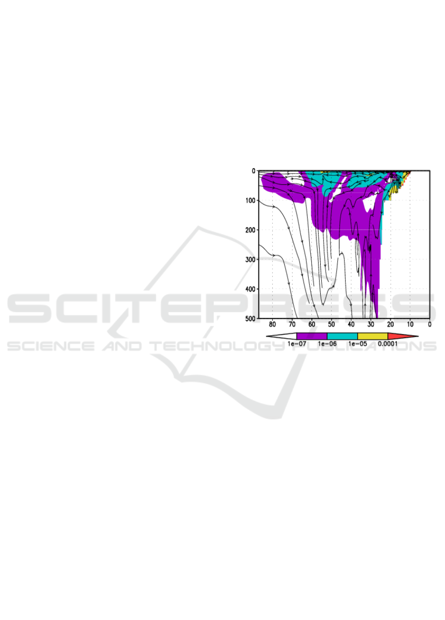
Figure 3: Pollution spreading vertical section normal to the

coast on the end of the model calculations on April 30,

2007, in the point near Sochi where pipe number 13 (Figure

2) is located. X-axis corresponds to the sea depth in m, y-

axes – distance in km.

Vertical section of total pollution spreading

normal to the coast on April 30, 2007, was made in

the point where pipe number 13 was located to study

vertical structure of pollution spreading from all the

rivers and pipes (Figure 3). Streamlines of currents

are plotted on the Figure 3, in order to estimate the

structure of pollution transport. According to the

presented figure, vertical pollution movement has an

advective character near the shore. In the coastal zone

along sea slope, pollution penetrates from the surface

to the deeper sea layers up to 500 m due to the

downwelling current. In the range of depths from 250

to 500 m the concentration of pollution has minimal

values. Due to the complicated eddy structure of

coastal currents complex 3-dimensional pollution

distribution is formed and pollutants travel significant

distances around 80 km. At a distance of 30-60 km

from the shore the pollution does not spread below

Numerical Modelling of the Circulation and Pollution Transport from Rivers and Wastewater Treatment Plants in the Sochi Coastal Area

381

250-100 m depths, as salinity halocline of the Black

Sea plays its locking role, preventing the ventilation

of the deep layers.

3.2 Laboratory Experiments

Several laboratory experiments studying

downwelling coastal current along a sloping bottom

were carried out at the Shirshov Institute of

Oceanology, Russian Academy of Sciences (IO RAS)

using special equipment: rotating tank with a cone in

the center of it. The results of experiments and

experimental setup are reviewed in detail in Elkin et

al., 2017.

This work showed that, in case of a sloping

bottom and in case of different densities of the water

in the tank and inflowing water, a bottom Ekman

layer was formed with a downward transport of less

dense water, which in turn experienced convective

instability.

The results of the performed laboratory

experiments were used to preliminary estimate

characteristics of the bottom Ekman layer on the shelf

of the Black Sea.

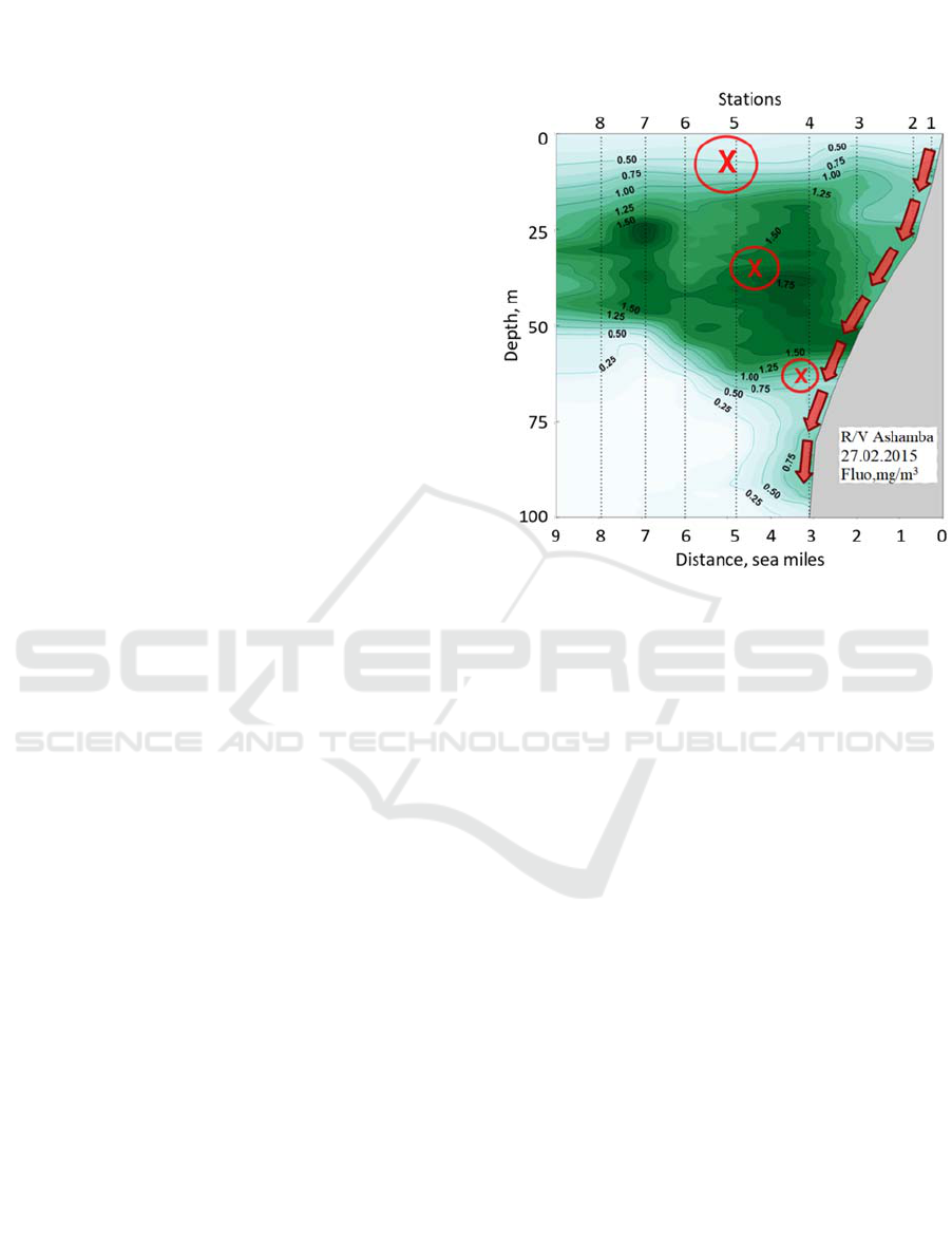
Field studies data (measurements of salinity,

temperature, pressure, and current velocity), collected

by the scientists from the IO RAS using the

autonomous Aqualog profiler at the Gelendzhik study

site from February 24, 2015 to March 2, 2015 were

used to analyze current structure in the coastal zone

at the study site of the Black Sea. Fluorescence

concentrations of chlorophyll a collected during the

monitoring of the Black Sea coastal zone on R/V

Ashamba on February 27, 2015, were also used to

study horizontal and vertical structure of pollution

spreading. Fluorescence concentrations of

chlorophyll a in upper 100 m layer in monitoring

transect is shown on Figure 4. X-sign on the Figure 4

corresponds to the current direction from us (in the

plane of the figure), so we can see alongshore current

in the coastal zone at the Gelendzhik study site, which

leads to the formation of the downwelling coastal

current in the Ekman bottom layer.

Following the estimates of the possible depth of

water sinking made in Elkin et al., 2017 and the

results on Figure 4, depth of less dense water

penetration is about 50 m. Moreover, waters with

small concentration of chlorophyll a can penetrate

lower than 100 m depth. Alternatively, according to

the work of Stanev (Stanev et al., 2013), ventilation

in the coastal zone spreads down to about 150–200 m.

These results were obtained from the analysis of

observations collected in the Black Sea from Argo

floats with oxygen sensors.

Corresponding numerical simulation results were

confirmed by laboratory experiments and observation

data.

Figure 4: Vertical section of chlorophyll a fluorescence

concentrations in the upper 100 m layer according to the

monitoring transect of R/V Ashamba in Black Sea coastal

zone on February 27, 2015, (Elkin et al., 2017). X-axis

corresponds to the sea depth in m, y-axes – distance in sea

miles.

4 CONCLUSIONS

We studied currents and the pollution transport in the

eastern coastal zone of the Black Sea using numerical

modelling technique. Proposed method makes it

possible to simulate not only large-scale structure of

the Black Sea circulation, but also the mesoscale and

sub-mesoscale dynamics of the coastal zone.

Results of the numerical modelling of coastal

dynamics and pollution spreading showed the effect

of vertical advection and water sinking in the Sochi

coastal area. Available experimental and

observational data from the works by Elkin et al.,

(2017) and Stanev et al., (2013) was used to validate

the results.

Reasonable, and in many cases good, agreement

between the numerical and experimental data

confirms the adequacy of the INMOM model in

reproducing horizontal and vertical structure of the

pollution spreading.

Future studies of the coastal dynamics and related

mechanisms of water sinking, vertical and horizontal

ONM-CozD 2019 - Special Session on Observations and Numerical Modeling of the Coastal Ocean Zone Dynamics

382

mixing of water will be conducted using numerical

modelling.

ACKNOWLEDGEMENTS

The presented work was supported by the Russian

Foundation for Basic Research according to the

research projects №18-35-00512, №17-05-41101.

REFERENCES

Diansky, N.A., 2013. Modelling of the ocean circulation

and study of its response to short-term and long-term

atmospheric forcing. 1

ed. Physmatlit, Moscow. (in

Russian)

Diansky, N.A., Fomin, V.V, Zhokhova, N.V., Korshenko,

A.N., 2013. Simulations of Currents and Pollution

Transport in the Coastal Waters of Big Sochi. Izvestiya,

Atmospheric and Oceanic Physics, 49(6): 611–621.

Dzhaoshvili, Sh.V., 1999. River runoff and sediment

transport to the Black Sea. Water Resources, 26 (3):

243–250.

Elkin, D.N., Zatsepin, A.G., Podymov, O.I., Ostrovskii,

A.G., 2017. Sinking of Less Dense Water in the Bottom

Ekman Layer Formed by a Coastal Downwelling

Current Over a Sloping Bottom. Oceanology, 57(4):

478–484.

Ivanov, V.A., Belokopytov, V.N, 2011. Oceanography of

the Black Sea. NAS of Ukraine, Marine Hydrophysical

Institute, Sevastopol. (In Russian)

Large, W., Yeager, S., 2004. Diurnal to decadal global

forcing for ocean and sea-ice models: the data sets and

flux climatologies. NCAR Technical Note, National

Centre for Atmospheric Research.

Pacanovsky R.C., Philander G., 1981. Parametrization of

vertical mixing in numerical models of the tropical

ocean. Journal of Physical Oceanography, 11: 1442-

1451.

Stanev, E.V., He, Y., Grayek, S., Boetius, A., 2013. Oxygen

dynamics in the Black Sea as seen by Argo profiling

floats. Geophysical Research letters, 40(12): 3085-

3090.

Numerical Modelling of the Circulation and Pollution Transport from Rivers and Wastewater Treatment Plants in the Sochi Coastal Area

383