Distributed Anomaly Detection of Single Mote Attacks in RPL Networks

Nicolas M. M

uller, Pascal Debus, Daniel Kowatsch and Konstantin B

ottinger

Cognitive Security Technologies, Fraunhofer AISEC, Garching near Munich, Germany

Keywords:

Intrusion Detection, IoT, Machine Learning, RPL.

Abstract:

RPL, a protocol for IP packet routing in wireless sensor networks, is known to be susceptible to a wide range

of attacks. Especially effective are ’single mote attacks’, where the attacker only needs to control a single

sensor node. These attacks work by initiating a ’delayed denial of service’, which depletes the motes’ batteries

while maintaining otherwise normal network operation. While active, this is not detectable on the application

layer, and thus requires detection on the network layer. Further requirements for detection algorithms are ex-

treme computational and resource efﬁciency (e.g. avoiding communication overhead) and the use of machine

learning (if the drawbacks of signature based detection are not acceptable). In this paper, we present a system

for anomaly detection of these kinds of attacks and constraints, implement a prototype in C, and evaluate it

on different network topologies against three ’single mote attacks’. We make our system highly resource and

energy efﬁcient by deploying pre-trained models to the motes and approximating our choice of ML algorithm

(KDE) via parameterized cubic splines. We achieve on average 84.91 percent true-positives and less than 0.5

percent false-positives. We publish all data sets and source code for full reproducibility.

1 INTRODUCTION

Wireless sensor networks (WSN) consist of a num-

ber of embedded devices, called motes, which have

a number of distinct characteristics. They run on

battery, communicate wirelessly, are comparatively

cheap, and thus have only very limited computational

capacity and memory. This is why they cannot run

the usual TCP/IP network stack, but use speciﬁcally

designed protocols such as RPL (Alexander, 2012).

RPL allows for routing between low-power devices

communicating via possibly lossy links. It has be-

come an industry standard due to its effectiveness.

Like all computer systems, motes are vulnerable

to cyber attacks. Coarse attacks such as jamming

shut down the network, which is why they are eas-

ily detected on the application layer. Additionally,

executing these attacks requires comparatively high

resources. Far more harmful are attacks such as Ver-

sion Number or Hello Flood, for which the attacker

only needs to control a single mote of the WSN (Wall-

gren, 2013). These attacks exhaust the batteries of the

motes in the WSN in a very short time and become

noticeable on the application layer only after the net-

work has already collapsed due to a lack of power

supply. Thus, it is very important to detect these at-

tacks already during the execution. Since the attacks

may vary, a generic anomaly detection system is de-

sirable, which is why machine learning (ML) tech-

niques may be useful. Additionally, detection has to

be extremely resource efﬁcient due to the motes’ very

limited resources.

In this paper, we present an anomaly detection

system suited to the requirements described above. In

summary, our contribution is as follows.

• We ﬁll a gap in existing research (see Section 2)

by presenting a ML-based system which can re-

liably detect single mote attacks such as Hello

Flood, Version Number, and Blackhole.

• We accommodate anomaly detection to a heavily

resource-constrained environment: We use pre-

trained models to avoid data collection and model

training on the motes, use a distributed architec-

ture to avoid communication overhead, and opti-

mize semi-supervised learning algorithms for low

computational overhead.

• We thoroughly evaluate our system by implement-

ing a prototype in C.

• We provide source code and data sets for repro-

ducibility

github.com/mueller91/single-mote-attacks

378

Müller, N., Debus, P., Kowatsch, D. and Böttinger, K.

Distributed Anomaly Detection of Single Mote Attacks in RPL Networ ks.

DOI: 10.5220/0007836003780385

In Proceedings of the 16th International Joint Conference on e-Business and Telecommunications (ICETE 2019), pages 378-385

ISBN: 978-989-758-378-0

 2019 by SCITEPRESS – Science and Technology Publications, Lda. All r ights reserved

2 RELATED WORK

There are multiple approaches for anomaly detection

in RPL-based WSNs. These can be classiﬁed accord-

ing to three criteria. First, anomaly detection can be

either machine learning (ML) based or signature/rule

based. Second, anomaly detection can be either cen-

tralized or decentralized. In a centralized system, ev-

ery mote sends the relevant data to a central mote,

mostly the RPL root mote which has a wired power

supply. A decentralized system runs in a distributed

manner, meaning that the data is processed on every

mote itself rather than sent to a central agent. Third,

anomaly detection in RPL-based WSNs can be cate-

gorized by its scope: The system may be designed to

detect anomalies in the payload data (layer 7 of the

OSI model), such as a deviation in the mote’s mea-

sured quantity, or to protect the WSN itself, for ex-

ample against attacks against its topology (layer 3).

Table 1 presents a summary of related work, clas-

siﬁed with the above criteria. While there are a num-

ber of anomaly detection systems for WSN, we ﬁnd

that there is a shortage of research on systems that

1. use machine learning to allow for detecting novel

attacks,

2. are decentralized, and

3. are designed to protect the WSN itself, e.g. detect

anomalies in layer 3.

We argue that such a system (ML based, decentral-

ized, on layer 3) is highly desirable due to the fol-

lowing reasons. First, since our goal is to detect

single-mote attacks as they occur, we need to dis-

cover these attacks on ISO-OSI layer 3. Second, cen-

tralized anomaly detection (where there is continuous

communication from the mote to the root) is not fea-

sible with battery powered devices. This is because

the process of sending data packets consumes a lot

of power compared to computation and data recep-

tion (D’Hondt, 2015). Finally, with the drawbacks of

signature based detection (expensive both in human

work and money, possibly not robust to small changes

in the attack pattern), a ML-based approach is highly

desirable. However, existing work which employs de-

centralized detection on layer 3 refrains, to the best of

our knowledge, from the use of machine learning (c.f.

Table 1). Thus, in the rest of this paper we present

such an approach.

3 RPL BACKGROUND

RPL is a layer 3 (ISO-OSI) protocol which provides

routing capabilities to low power devices communi-

Table 1: Work on anomaly detection (AD) on RPL-based

WSNs, categorized by detection method (ML: Machine

Learning based, S: Signature based), agent positioning (c:

centralized, dc: decentralized) and detection scope with re-

spect to OSI Layer model.

Summary

Methodol-

ogy / Type

/ Layer

Evaluation of various models on

synthetically-created payload (layer 7)

data. (Bosman, 2016)

ML / dc / 7

Distributed KNN for payload data AD,

minimizes communication by

clustering sensor measurements.

(Rajasegarar et al., 2006)

ML / dc / 7

Clustering based, partitions data space

using fuzzy C-means algorithm in an

incremental mode. (Kumarage et al.,

2013)

ML / dc / 7

Centralized, detects Selective

Forwarding Attacks using SVMs and

sliding windows. High communication

overhead. (Kaplantzis et al., 2007)

ML / c / 3

Centralized via Neural Net running on

a Desktop PC. (Almomani et al., 2016)

ML / c / 3

Signature-based approach on all

network stack layers. (Bhuse and

Gupta, 2006)

S / dc / 3

Detects set of pre-deﬁned attacks using

a combination of signature-based

approaches. (Raza et al., 2013)

S / dc / 3

Rule-based detection using separation

of motes into guard nodes and

communication nodes. (Hoang et al.,

2015)

S / dc / 3

cating over lossy links. Starting from a single root

node (which usually has a wired power and internet

connection), RPL constructs a Destination Oriented

Directed Acyclic Graph (DODAG). This is a usually

tree-like structure where the root is the wired node

and the wireless motes are the internal nodes and

leaves. In order to track changes, a DODAG version

number is used. If the DODAG version number in-

creases, the DODAG will be reconstructed. Messages

can be sent from the wireless motes by forwarding

messages upwards in the direction of the root. Motes

may change their parents, based on the optimization

of various parameters such as energy consumption or

loss (Alexander, 2012). Each node determines its par-

ents based on their rank, which is calculated based on

the objective function and can be viewed as an ab-

stract distance from the root node. Fig. 1 shows an

example of such a topology. RPL has been designed

to be very resource efﬁcient, and introduces routing

capabilities to tiny devices which are unable to run

the full TCP/IP stack (Alexander, 2012).

Distributed Anomaly Detection of Single Mote Attacks in RPL Networks

379

Figure 1: Example of a WSN topology, where the RPL pro-

tocol has created a DODAG connecting the WSN’s motes to

the root mote (node 0). An arrow connecting two motes in-

dicates a child-parent relationship. Any mote can send data

to the root by sending a packet to its parent, which in turn

forwards it to its parents, until the packet reaches the root.

4 ATTACK SCENARIO

In this Section we present the attack scenario consid-

ered in this paper. For this, we will ﬁrst deﬁne the

threat model specifying the theoretical capabilities of

the attacker and then shortly explain three representa-

tive attacks which are used for evaluation.

4.1 Threat Model

Different threat models on WSNs can be distin-

guished by how powerful the attacker is. For example,

if the attacker has free access to the area where the

WSN is located, he can place a jammer that blocks

the medium and all communication of the WSN (De-

nial of Service). However, the WSN may be located

in a closed area, e.g. a factory building, to which the

attacker has no easy access. If the attacker is able to

control a larger number of motes, he can achieve simi-

lar effects to jamming, e.g. by network segmentation.

However, this scenario is often not realistic either, and

the attacker may be limited to introducing very few or

only a single malicious mote into the network. This

is the case, for example, with more extensive physical

access controls, where the attacker has to take over or

smuggle in motes at high cost. The rest of this paper

is based on this threat model: The attacker controls

exactly one mote (malicious mote) of the entire WSN

and his goal is to cause as much damage as possible

with these very limited resources.

4.2 Evaluated Attacks

A number of single mote based attacks on RPL are

known, but nearly all are variations of DIO ﬂooding,

illegitimate version number increase, or rank spoof-

ing. Thus, we chose three representatives of these

build blocks to evaluate our system against. (Pongle

and Chavan, 2015)

• Version Number Attack. This attack increases

the version number, forcing unnecessary graph re-

buildings. This attack affects the availability of

the network, since the additional overhead drains

the nodes’ batteries.

• Hello Flood Attack. A ﬂooding attack, causing

nodes within range to send large amounts of re-

sponse packets. The attacker’s goal is to affect

availability by making the network unstable and

causing the sensor nodes to rapidly deplete their

batteries.

• Blackhole Attack. This attack establishes a Sink-

hole by advertising a very low rank, making itself

very attractive to surrounding motes. These con-

sequently select the malicious mote as their par-

ent, resulting in all of their trafﬁc ﬂowing through

the attacker, who may then choose to drop all

packets (Blackhole) or only a few selected (Grey-

hole).

5 SYSTEM OVERVIEW

In this Section we present our system in detail. It con-

sists of the following steps.

First, every node pipes the packages it receives to

the anomaly detection engine, where appropriate fea-

tures are extracted (see Section 5.1). Second, a pre-

trained model is selected depending on the number

of nodes in the node’s communication range (Sec-

tion 5.2). Third, the model is evaluated on new data

points as they come in. If the anomaly score falls

below a pre-deﬁned threshold α, the system sends

an anomaly notiﬁcation packet to its neighbors via

broadcast, which the receiving nodes forward to the

root. We detail these steps in Section 5.3. We now

proceed to illustrate the individual steps in detail.

5.1 Feature Construction

For security anomaly detection in RPL-based WSNs,

we construct the following features, which are con-

structed on every node in the network topology inde-

pendently.

Count of DIS, DIO and DAO Packets. Over a

window of 15 seconds we aggregate the number of

DODAG Information Solicitation (DIS), DODAG In-

formation Object (DIO), and Destination Advertise-

ment Object (DAO) packets a node receives.

SECRYPT 2019 - 16th International Conference on Security and Cryptography

380

Number of DODAG Versions. Over a window

of 500 seconds we count the number of different

DODAG versions.

UDP forward Ratio. Deﬁne the neighborhood

N(m) of a node m to be the set of nodes in the WSN

that are within communication range of m. For all

o ∈ N(m), let to(o, m) be the number of UDP pack-

ets sent to a given node o as observed by m, and let

f rom(o, m) be the number of UDP packets sent from

o observed by m.

Note that m may not observe all UDP packets sent

to o due to communication range limitations, but is

guaranteed to observe all packets sent from o, since

they are in communication range (except for inherent

packet loss due to the network’s lossy links). We de-

ﬁne the maximum UDP forward ratio as

r(m) := max

o∈N(m)

to(o, m)

from(o, m)

. (1)

Intuitively, every node m takes note how the nodes

in its neighborhood forward UDP packets. If a given

node receives a lot of packets, but forwards none or

only very few, this may indicate a Blackhole attack.

We chose these features because ﬁrst, we consider

them to carry meaningful information about the sta-

tus of our network, and second because feature selec-

tion via grid search has shown that these features are

indeed the most useful for detecting network anoma-

lies.

5.2 Model Construction and Selection

In this subsection, we describe our choice of ML

model. We especially consider how to minimize com-

putation and memory consumption once the model is

deployed to the sensor nodes.

5.2.1 Model Selection

The foundation of our anomaly detection system is

Kernel Density Estimation (KDE), a technique to ap-

proximate a density function f . We choose this model

because of the following reasons. First, it offers some

degree of probabilistic explainability: Given a thresh-

old, KDE returns a range of ’normal’ and ’anomalous’

values together with the corresponding probabilities,

which may help network operators to better under-

stand the nature of anomalies that occur. SVM allows

only for distance-based explainability, while Auto-

Encoders provide none. Second, KDE is adaptable to

heavily resource constrained environments (see Sub-

section 5.2.3). We refrained from using other poten-

tially interesting models such as an Auto-Encoder or

HMM due to the following reasons.

1. HMMs are not easily adaptable to a heavily re-

source constrained environment such as sensor

motes. This is because the necessary inference

algorithm (the ’forward algorithm’) has complex-

ity θ(nm

) (where n is the sequence length and m

the number of hidden variables). This exceeds the

computations necessary if spline-approximated

KDE is used (see Section 5.2.3).

2. While Auto-Encoders (AE) are useful for

anomaly detection in general, they are ill suited

to our task due to the following reasons. First, the

computation of nonlinearities such as tanh or exp

requires the evaluation of several higher order

polynomials (Pad

e approximation), which ex-

ceeds the computational complexity of evaluating

a cubic spline as is required in our approximation

of KDE (Section 6.3). Second, the reconstruction

error δ is not directly interpretable as a probability

distribution, which we require as described in

Section 6.3.

5.2.2 KDE Background

We chose KDE as our anomaly detection algorithm.

Given a set of N i.i.d. drawn samples x

, KDE yields

an estimator

f which is given by the following sum

of scaled and translated kernel functions k (usually

Gaussians):

(x) =

∑

i=1



x−x



. The bandwidth

parameter h balances out the estimator’s bias and vari-

ance. We make the simplifying assumption that each

data point x

∈ R

is independent from all other data

points x

∈ R

, i 6= j and that all D features are inde-

pendent from each other.

Since our data consists of multivariate vectors

x = [x

, .., x

]

, we adapt univariate KDE as follows:

For each feature x

, we train and evaluate a univariate

KDE

. A multivariate data point x is then scored

by the sum of the log-likelihood of the individual

s(x) =

∑

d=1

log(

)). This implicitly assumes that

the features are independent, but avoids the require-

ment to use multivariate KDE, for which the opti-

mizations in Section 5.2.3 are infeasible. The hyper-

parameter h is found using parameter optimization as

follows: Given a data set X, we split it into a training

and a validation set. For a set of real numbers H , for

each h ∈ H , we ﬁt

to the training set and evalu-

ate on the validation set, thus ﬁnding a parameter h

which maximizes s(x).

5.2.3 KDE in a Resource Constrained

Environment

While KDE is a suitable approach to our problem,

it has its downsides. For example, the evaluation of

Distributed Anomaly Detection of Single Mote Attacks in RPL Networks

381

f (x) given a new sample x is very expensive, since

for N data points and D features each kernel function

k has to be evaluated and summed up. Computational

complexity and memory consumption are in O(N · D)

and thus prohibitively expensive. To mitigate these

issues, we modify our model as follows.

Model Pre-training. Instead of training our

model on the sensor nodes, we ﬁrst collect training

data (see Section 6.1 for details) and train our model

on a desktop computer. The training data X con-

sists of the log ﬁles from motes. These include the

features as deﬁned in Section 5.1. From the logs

we extract subsets P

(m) containing features based

on those packets sent by node m and its neighbors.

Neighbors of node m are all nodes that are within

communication range of m. Let l be the maximal

number of neighbors in the desired WSN. Then, for

j = 1, ..., l, let X

be the union of all data points of

all P

(m) where m has exactly j neighbors. Finally,

we ﬁt a KDE to each X

as described above. Thus, we

obtain up to l models, parameterized by the number of

neighbors. We will thoroughly evaluate this approach

in Section 6.

Spline Approximation. Next, we approximate

our density estimate

f using a third-order spline. This

is a function deﬁned piecewise by third-order poly-

nomials. Let m

be the maximum value of a given

feature x

in the training data. We approximate

in the interval [0, m

] using k subintervals. Outside

the interval we extrapolate by quadratically decreas-

ing the function, thereby mimicking KDE’s summa-

tion of normal distributions. Let x

border

be the value

of the border of feature d at which we want to extrapo-

late. Then our extrapolation is given by the following

equation:

log(

)) ≈ −

− x

border

)

+ log(

border

)).

Note that the computational cost of this approxima-

tion is in O(D), and the disk space required is only in

O(D · l · k), where l ·k is much smaller than N.

Finally, we deploy all up to l spline approxima-

tions to the sensor node. The node periodically checks

how many neighbors it has, and chooses the appropri-

ate spline to evaluate new data points. If, for some

reason, no model for j neighbors has been trained, the

node substitutes with a model for j

neighbors such

that | j − j

| is minimized.

5.3 Anomaly Detection Workﬂow

We now proceed to describe the complete anomaly

detection system. First, we begin with the model

training, which is as follows (see Fig. 2):

Figure 2: Workﬂow of the model up to deployment.

1. Collect logs from a normally operating WSN.

2. Partition training set by number of neighbors.

Create the training sets X

, establishing a base-

line for what a node with j neighbors can expect

a normally functioning RPL network to look like.

3. Model training. For each such training set and

every feature, train a univariate KDE and ﬁnd the

optimal bandwidth using grid-search.

4. Model Compression. Approximate every log-

KDE density using a univariate cubic spline.

5. Model deployment. Deploy splines to each mote.

The detection workﬂow is as follows (see Fig. 3):

1. Evaluate anomaly score at all nodes. Evaluate

incoming data using score function s from Sec-

tion 5.2.1, where

is replaced by its spline ap-

proximation.

2. Notify neighbors in case of an anomaly. If the

score is less than a given threshold T , the current

status of the node is considered anomalous. The

node then proceeds to send anomaly notiﬁcation

packets (ANP) to all neighbors, which in turn for-

ward them to the root.

3. Evaluate ANP at root. If the root receives ANPs

from more than a certain number of motes, it can

raise an alert.

We focus on detecting anomalies, thus sending ANPs

is currently not implemented.

SECRYPT 2019 - 16th International Conference on Security and Cryptography

382

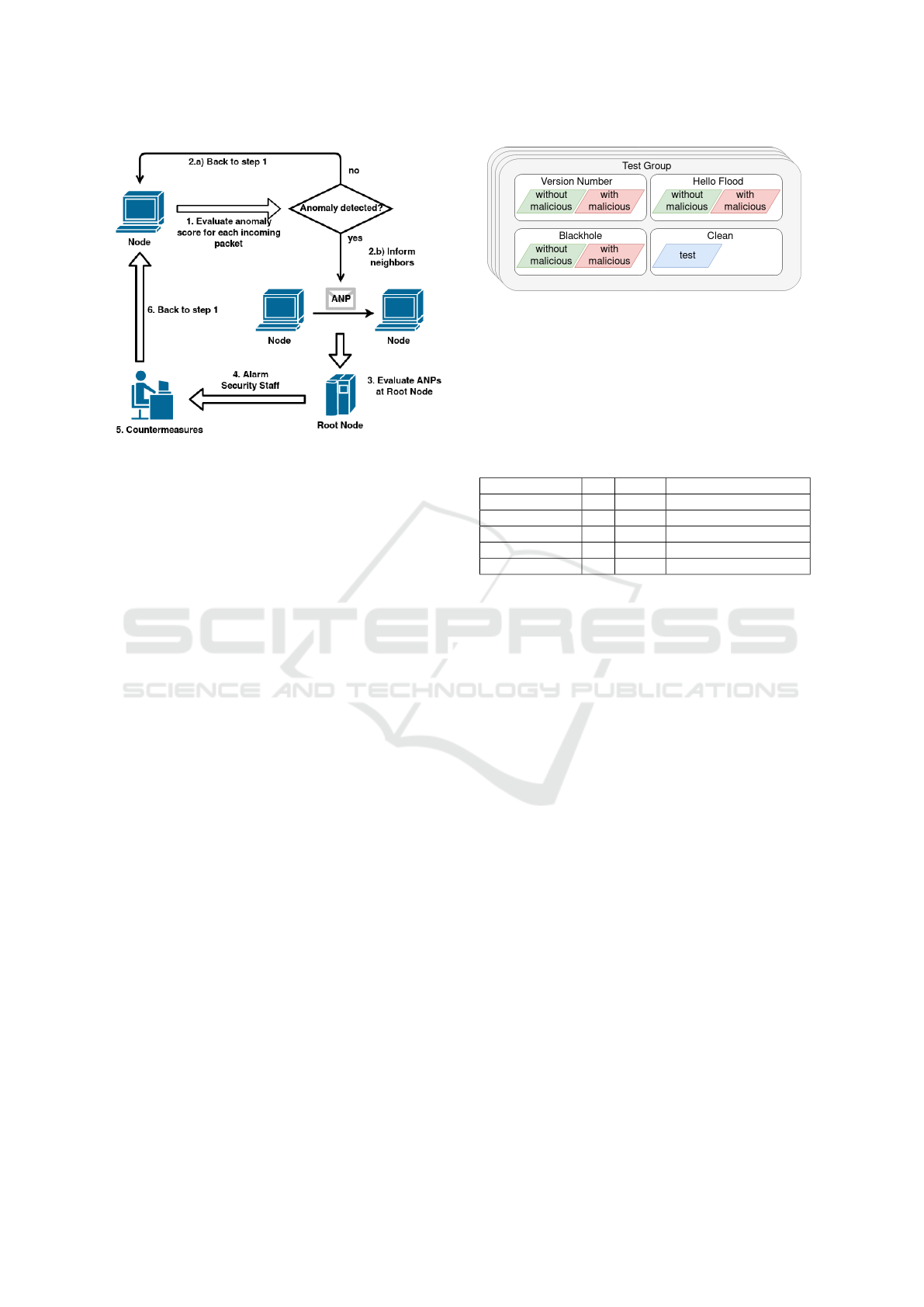
Figure 3: Anomaly detection workﬂow.

6 IMPLEMENTATION AND

RESULTS

In this Section we present our data sets, details of

our implementation, and preliminary results. In our

implementation, we use H = numpy.logspace(-4, 4,

num=25), T = −23.88 for τ = 1% FP in the training

set, l = 5 and k = 5.

6.1 Data Sets

All data used in this project is obtained by simulat-

ing RPL-based networks in the Cooja network sim-

ulator (Dunkels et al., 2004). In order to simulate

the attacks, we use a modiﬁed version of the RPL At-

tacks Framework (D’Hondt, 2015). We create 20 test

groups comprising 80 individual data sets, as shown

in Table 2. Each data set consists of two sub data sets:

One with and one without malicious node. We call

the former malicious, the latter non-malicious data

set. The only exception to this is the Clean set, which

consists of a single non-malicious set we call test set.

The reason for this separation will become apparent

in Section 6.2. Each of these sub data sets contains

all features based on packets received throughout the

simulation. See Fig. 4 for a visual representation of

this.

6.2 Implementation

We implement our system in C using Contiki OS

and Cooja to simulate Zolertia Z1 motes with

MSP430X series CPU. We train exclusively on the

non-malicious data, test on the malicious data, and

use the Clean data to evaluate the false positive rate.

Figure 4: Layout of the data we use. There are 20 Test

Groups, each containing four data sets. Except for the Clean

set, each data set contains two subsets, one with malicious

node and one without.

Table 2: Overview of the data sets we use for evaluating our

system. Each Test Group contains four individual data sets,

as shown in Fig. 4. The topology (r)ectangle is a pre-deﬁned

grid, neighbors, (q)uadrants is a completely random layout

and (g)rid arranges the motes in layers around the root mote.

M denotes the number of nodes in the simulation.

Test Group Nr. M Topo. Simul. duration [sec]

1, 2, 3, 4 7 (r) 800, 1000, 1200, 1400

5, 6, 7, 8 7 (q) 800, 1000, 1200, 1400

9, 10, 11, 12 12 (q) 800, 1000, 1200, 1400

13, 14, 15, 16 9 (g) 800, 1000, 1200, 1400

17, 18, 19, 20 12 (g) 800, 1000, 1200, 1400

6.3 Anomaly Threshold

The selection of the anomaly threshold is a common

problem in the ﬁeld of anomaly detection which we

approach statistically, using test theory. As described

in Section 5.3, the detection workﬂow has two stages:

Anomaly scoring at mote-level and anomaly notiﬁca-

tion packets (ANP) evaluation at the root-level where

the ﬁnal alert decision is made. This leads to one

threshold T for the mote-level detection and a min-

imal number of ANPs threshold k at root-level. In

the following, we deﬁne T to be the τ-percentile of

our non-malicious data scores which results, by deﬁ-

nition, in a false positive rate of τ for the mote-level

detectors. In statistical tests, the maximum accept-

able probability of a false positive (Type I error) is

known as signiﬁcance level. Hence, τ can be inter-

preted as such. To determine the critical number of

ANPs, we employ the following binomial test: Let

be a random variable representing the number of

ANPs received in a time slot t and n the number of

nodes in the network. We use the simplifying assump-

tion that, in the absence of an attack, motes send an

ANP with probability p independently of each other

such that X

follows a binomial distribution B(n, p)

for all t. We formulate the null hypothesis H

: p = τ

which means that the observed realization of X

solely due to the introduced false positive rate τ. The

alternative, H

: p > τ, can therefore be interpreted

Distributed Anomaly Detection of Single Mote Attacks in RPL Networks

383

Table 3: Size of the motes with anomaly detection and with-

out anomaly detection. Column 2 shows the size of the text

segment, column 3 of the data segment, column 4 of the bss

segment, and column 5 shows the total size.

text data bss dec

without AD 47099 348 4652 52099

with AD 53405 2148 5370 60923

as the result of an attack. Assuming a signiﬁcance

level of α, the threshold k can then be determined by

demanding that P(X

≥ k|p = τ) =

∑

j=k

B( j; n, p) =

∑

j=k





n− j

(1 − p)

≤ α. In our implementation we

choose the common value of 0.01 for both signiﬁ-

cance levels τ and α resulting in a critical ANP num-

ber of k = 2. Of course it would be desirable to be

able to choose τ and α as low as possible, however,

as known from test theory, this comes at the cost of

higher false negative (Type II error) probability.

6.4 Results

When we implement and evaluate this pipeline as de-

scribed in Section 5.3, we obtain the following results.

On average, our system detects the Blackhole, Hello-

Flood and Version Number attacks with 68%, 90%

and 96% true positives respectively, and 0.5% false

positives. Table 4 details these results. Also note that

the detection on mote level is implemented in C, but

sending ANPs (and therefore, detection on root level)

is currently simulated in a python script.

In the Blackhole attack scenario, the degree to

which the attacker manages to establish themselves

as a parent of the surrounding nodes varies signiﬁ-

cantly. This is due to the random layout of the topol-

ogy, where the malicious node may be placed un-

favourably for the attacker. We indicate this ’degree

of success’ of the black hole attack by the malicious

UDP ﬂow ratio increase, which is the increase in UDP

packets received by the malicious node in comparison

to an ordinary mote. For example, in data set 20, the

malicious note receives less than 1% additional traf-

ﬁc compared to an average mote, i.e. the black hole

attack can not be considered effective. Consequently,

there is a very low detection rate (less than 5%). In

contrast, the attack is very effective in data set 1 (ma-

licious UDP ﬂow increased by 550%), which results

in a detection rate of 91%.

6.5 Security Considerations

In this Subsection, we brieﬂy examine to which extent

the attacker can circumvent our anomaly detection if

he knows that it is employed in a given WSN. First,

we consider avoiding detection on the mote level. As

Table 4: Results of our anomaly detection system on all Test

Groups, where the system was trained on the non-malicious

data from all Test Groups. The tables details the false posi-

tive rate for the Clean Set, and the true positive rate for the

Blackhole, Hello Flood and Version Number attack. For the

black hole attack, ’UDP ﬂow’ indicates the increase of UDP

packets to the attacker in comparison to an average node.

Clean Blackhole H.F. V.N.

FP TP

UDP

Flow

TP TP

1 0.0% 91.8% +554% 91.1% 95.0%

2 0.5% 87.4% +413% 91.9% 95.5%

3 0.0% 95.0% +542% 97.9% 96.6%

4 0.7% 90.3% +570% 96.4% 96.4%

5 0.0% 82.9% +370% 93.0% 96.2%

6 0.0% 85.4% +270% 91.9% 97.5%

7 0.0% 76.5% +204% 93.7% 95.8%

8 0.4% 12.6% +67% 94.6% 95.7%

9 0.0% 35.4% +167% 90.5% 97.5%

10 5.1% 77.8% +377% 87.9% 93.9%

11 0.0% 45.4% +319% 92.0% 96.2%

12 0.4% 83.5% +566% 83.8% 98.6%

13 0.0% 73.4% +496% 82.3% 94.3%

14 0.0% 89.9% +555% 82.3% 96.0%

15 0.0% 76.5% +485% 94.1% 97.9%

16 0.7% 57.2% +269% 89.6% 93.9%

17 1.9% 73.4% +470% 77.9% 96.8%

18 0.0% 75.3% +505% 88.4% 98.5%

19 0.0% 56.3% +368% 92.9% 97.1%

20 0.4% 4.7% +0.1% 91.4% 91.7%

All 0.5% 68.52% +379% 90.2% 96.1%

for the Hello Flood and Version Number attack, there

is no way to evade detection, because these attacks

work intrinsically by ﬂooding the network, which

cannot be hidden from the anomaly detection what-

soever. Also, since the model comes pre-trained, the

possibility of a ’concept drift’ is ruled out, e.g. the at-

tacker slowly getting the network used to an increase

of trafﬁc. As for the Black Hole attack, the attacker

can trade off effectiveness against stealthiness. This

is achieved by transitioning to a ’Grey Hole’ which

blocks some messages while forwarding others. Ob-

viously, this also decreases the impact of the attack.

There are scenarios in which the attack may modify

the trafﬁc before forwarding, thus possibly avoiding

detection while also violating the network’s integrity.

This, however, is not detectable on ISO-OSI layer 3,

and requires layer 7 packet checking, which is out of

the scope of this work.

Second, we consider avoiding detection on the

root level, e.g. preventing or diminishing the impact

of ANPs sent by individual motes. Spooﬁng an in-

creased number of nodes does not reduce the detec-

tion chances, since it is only used in the hypothe-

SECRYPT 2019 - 16th International Conference on Security and Cryptography

384

sis test and there the number of nodes is deﬁned by

the network administrator. Alternatively, the attacker

may try prevent ANPs reaching the node by means

of a black hole, simply dropping all incoming traf-

ﬁc. Our system tries to mitigate this by broadcasting

ANP packets instead of sending them directly to the

root, thus potentially ﬁnding an alternate path of tran-

sit which does not comprise the malicious mote.

6.6 Model Overhead

Since WSN motes have limited memory, we evaluate

the memory overhead of our system in this Section.

We compare a Z1 mote with our anomaly detection

system against a Z1 mote without our anomaly detec-

tion system. For this, we use the unix size command.

The results are given in Table 3.

The results indicate that the addition of our system

increases the size of the executable by around 17%.

The text section increases by 13% and is the largest

absolute contributor to the size increase. data and bss

sections increase by less than 2000 bytes.

Since the mote’s computational power is also very

limited, we evaluate the additional time required for

the added functionality. The time is measured in clock

ticks given by Contiki’s RTIMER NOW function. In

the Zolertia Z1 motes, the corresponding clock has

ticks per second. For initialization of our algo-

rithm, a node requires on average 197.81 ticks. This

corresponds to 6.04 milliseconds. Frequently called

tasks take on average 208.23 ticks per second and,

thus, take less than 0.64% of the CPU time each sec-

ond. Additionally, we have to modify the packet pro-

cessing of the network stack leading to an increase of

the average time for processing a packet from 22.79

ticks to 25.77 ticks, which corresponds to an increase

of 13.04%.

7 CONCLUSION

In this paper, we present an anomaly detection sys-

tem which is designed to detect single mote attacks

on RPL based-networks on layer 3. This is impor-

tant with these kinds of attacks since they can only

be detected on the application layer after the dam-

age has already been dealt. We implement our system

in C, evaluate it against a set of different topologies,

and show that it can reliably detect three fundamen-

tal attack types while at the same time respecting the

motes’ energy and storage constraints.

REFERENCES

Alexander, R. (2012). RPL: IPv6 Routing Protocol for Low-

Power and Lossy Networks. RFC 6550.

Almomani, I., Kasasbeh, B. A., and Al-Akhras, M. (2016).

WSN-DS: A Dataset for Intrusion Detection Sys-

tems in Wireless Sensor Networks. J. Sensors,

2016:4731953:1–4731953:16.

Bhuse, V. and Gupta, A. (2006). Anomaly intrusion detec-

tion in wireless sensor networks. J. High Speed Netw.,

15(1):33–51.

Bosman, H. H. W. J. (2016). Anomaly detection in net-

worked embedded sensor systems. PhD thesis, Tech-

nische Universiteit Eindhoven.

D’Hondt, A. (2015). RPL attacks framework. Tech-

nical report, Universit catholique de Louvain.

https://github.com/dhondta/rpl-attacks/.

Dunkels, A., Gronvall, B., and Voigt, T. (2004). Contiki - a

lightweight and ﬂexible operating system for tiny net-

worked sensors. In 29th Annual IEEE International

Conference on Local Computer Networks, pages 455–

462.

Hoang, H. T., Eui-Nam, H., and Minho, J. (2015). A

lightweight intrusion detection framework for wire-

less sensor networks. Wireless Communications and

Mobile Computing, 10(4):559–572.

Kaplantzis, S., Shilton, A., Mani, N., and Sekercioglu,

Y. A. (2007). Detecting selective forwarding attacks

in wireless sensor networks using support vector ma-

chines. In ICISSNIP 2007, pages 335–340.

Kumarage, H., Khalil, I., Tari, Z., and Zomaya, A. (2013).

Distributed anomaly detection for industrial wireless

sensor networks based on fuzzy data modelling. Jour-

nal of Parallel and Distributed Computing, 73(6):790

– 806.

Pongle, P. and Chavan, G. (2015). A survey: Attacks on

RPL and 6lowpan in IoT. In 2015 International Con-

ference on Pervasive Computing (ICPC). IEEE.

Rajasegarar, S., Leckie, C., Palaniswami, M., and Bezdek,

J. C. (2006). Distributed anomaly detection in wire-

less sensor networks. In 2006 10th IEEE Singapore

International Conference on Communication Systems.

Raza, S., Wallgren, L., and Voigt, T. (2013). SVELTE:

Real-time intrusion detection in the internet of things.

Ad Hoc Networks, 11(8):2661 – 2674.

Wallgren, L. (2013). Routing Attacks and Countermeasures

in the RPL-Based Internet of Things. International

Journal of Distributed Sensor Networks, 9(8):794326.

Distributed Anomaly Detection of Single Mote Attacks in RPL Networks

385