
Disturbance Observer for Path-following Control of Autonomous
Agricultural Vehicles
T. Hiramatsu, M. Pencelli, S. Morita, M. Niccolini, M. Ragaglia and A. Argiolas
Yanmar R&D Europe S. R. L., Viale Galileo 3/A, Firenze, Italy
Keywords: Path-following Control, Agricultural Tractor, Disturbance Observer.
Abstract: This paper proposes a disturbance observer to be integrated inside a path-following controller in order to
improve motion accuracy of an autonomous driving tractor. During operation, the tractor undergoes the effects
of external forces due to either the action of the implement or the inclination of the ground. In such conditions,
it is difficult to work precisely along a pre-determined path. By considering external forces as disturbances,
it is possible to design a disturbance observer that estimates the steering angle on the basis of yaw-rate and
lateral velocity. The proposed approach has been tested in a simulation environment.
1 INTRODUCTION
With rises in global population comes the problem of
food shortages. For instance, in Japan the number of
farmers is decreasing and farmers are rapidly aging
(Noguchi and Barawid, 2011). In the near future, this
situation will likely result in shortages in food
production. Eventually, the same issue is expected to
happen all over the world (Blackmore, 2009), (Ball et
al, 2017). For these reasons, automation technologies
such as autonomous driving are needed to work large
fields with fewer farmers. One of the most relevant
problems in automated agriculture consists in
controlling a machine along a predetermined path, in
presence of rough terrain or inclined ground.
Furthermore, the presence of ridges requires
agriculture vehicles to move within 5.00-10.00 cm
accuracy with respect to the predetermined path.
Unfortunately, the presence of the implement and
also the effect of gravity on inclined fields typically
introduce disturbance effects that prevent the
machine to achieve the required accuracy. Moreover,
motion accuracy is influenced by soil conditions,
which in turn depend on geographical location,
climate and other environmental factors.
Even though, in principle, it would be possible to
accurately model slip phenomena by taking into
account all the aforementioned factors, the resulting
model would almost surely be too complex to be used
for control purposes. For this reason, rather than
focusing on the physical modelling of these
disturbances, the research community spent a
significant effort in developing compensation
strategies to overcome the effects of slip phenomena
and to improve motion accuracy. Several solutions
based on Kalman filtering have been proposed, like
for instance (Shalal et al, 2013), (Pentzer et al, 2014),
(Lenain et al, 2004), (Fang et al, 2005). Alternative
approaches relying on both dynamic models and
Kalman filtering proved to be effective in estimating
slipping or, alternatively, in identifying the resulting
variation of the instantaneous centre of rotation.
However, the main limitation of these approaches
consists in limited robustness with respect to rapidly
changing soil conditions. More recently, techniques
based on disturbance observation have been proposed
to solve these problems, like for instance (Wen-Hua
et al, 2016) and (Hyungbo et al, 2016). More in detail,
the disturbance observer (DOB) consists in an inner-
loop controller, whose primary role is just to
compensate uncertainties in the plant and exogenous
process disturbances. Several applications of DOB to
the control of autonomous vehicles can be found in
the scientific literature. For instance, in (Nguyen et al,
2014) the authors propose a DOB to estimate the
vehicle’s yaw angle using low-cost sensors. While
being based on a rather simple kinematic car-like
model, this solution is actually able to improve the
controller’s accuracy by reducing the lateral error
with respect to the pre-defined path. In (Huang and
Zhai, 2015), a DOB is applied to estimate exogenous
disturbances acting on a wheeled mobile robot. In
(Taghia and Katupitiya, 2013), a sliding mode
controller is designed with DOB for a farm vehicle.
Hiramatsu, T., Pencelli, M., Morita, S., Niccolini, M., Ragaglia, M. and Argiolas, A.
Disturbance Observer for Path-following Control of Autonomous Agricultural Vehicles.
DOI: 10.5220/0007834402510258
In Proceedings of the 16th International Conference on Informatics in Control, Automation and Robotics (ICINCO 2019), pages 251-258
ISBN: 978-989-758-380-3
Copyright
c
2019 by SCITEPRESS – Science and Technology Publications, Lda. All rights reserved
251
The DOB eliminates the chattering of sliding mode
control and compensates the system uncertainties. A
different approach is proposed in (Rathgeber et al,
2015), where the authors face the problem of lateral
trajectory tracking control of an autonomous driving
car. A DOB-based controller that rejects external
forces has been adopted in (Yu et al, 2018) in order to
compensate the effect of cross-wind on the motion of
a 4-wheel steering vehicle. However, this approach
does not take into account the path-tracking problem
and it also lacks versatility since it relies on extensive
tuning of both controller and observer gains.
In this paper, we propose a DOB-based path-
following control algorithm able to improve the
accuracy of an autonomous agricultural tractor in
terms of lateral error with respect to a pre-defined
path. The external forces originating either from the
action of the implement or from the inclined ground
are directly considered as disturbances. The proposed
DOB combines the yaw-rate and the lateral velocity
of the vehicle to reject the exogenous disturbances.
As a result, the main advantages of this approach
consist in eliminating the need to re-tune control
gains whenever soil conditions change. The
remainder of the paper is structured as follows:
Section 2 introduces the proposed control system,
while Section 3 describes the adopted dynamic
model, and the DOB’s transfer function is analysed.
Finally, simulation results are shown in Section 4.
2 PATH-FOLLOWING CONTROL
AND PROBLEM DEFINITION
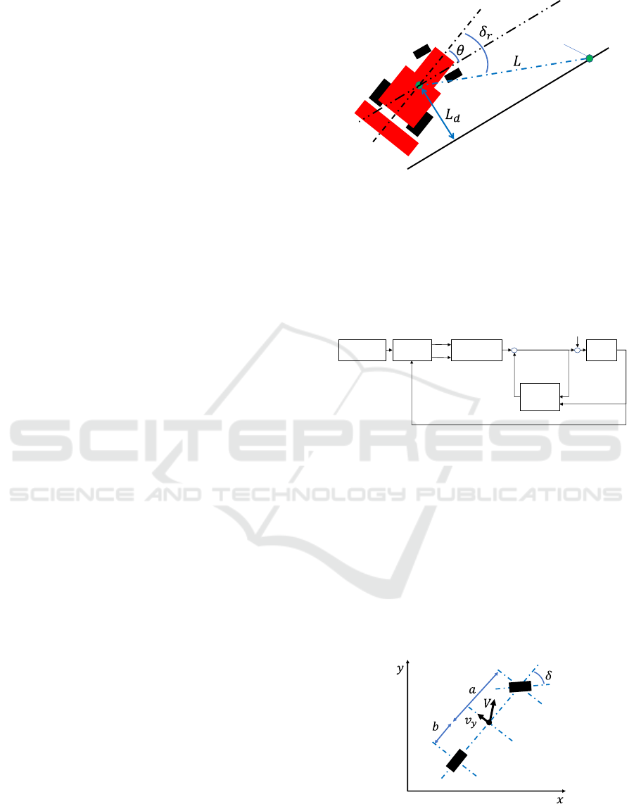
First of all, let us introduce the autonomous control
scheme for the agricultural tractor shown in Figure 1.
We here consider a simple path-following control
scheme, where θ is the heading angle error,
is the
lateral error with respect to the path, and L is the look
ahead length. More specifically, L is defined as the
distance between the current position of the machine
and a specific point on the reference path, named
“look-ahead point”. By choosing a constant value of
L, the look-ahead point can be computed accordingly
as shown in (Samuel et al, 2016). Therefore, the target
steering angle
can be defined as:
For the sake of clarity, the reference path is defined
in advance on the basis of several specifications
provided by farmer (namely the geometry of the field,
the kind of implement, the size of the tractor, etc.).
Figure 1: Autonomous control scheme.
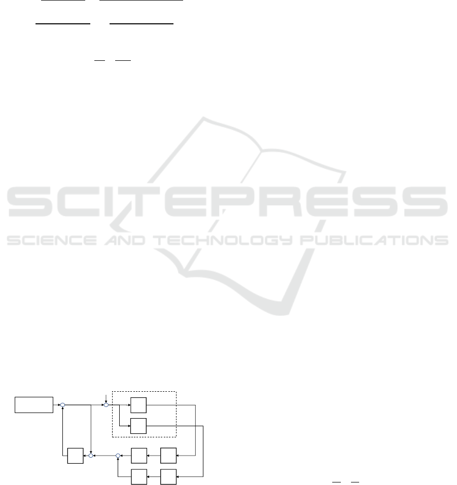
Please notice that, at this stage, the controller does not
take into account any disturbance. Therefore, it is not
able to guarantee adequate motion accuracy while
working on the agricultural field. In order to solve this
problem a DOB is introduced, leading to the
architecture displayed in Figure 2, where d is
disturbance used for compensation.
Figure 2: Block diagram of closed loop system.
3 DISTURBANCE OBSERVER
DESIGN
We describe the tractor kinematics using the single-
track model shown in Figure 3, where, and are the
distances from the center of gravity position (CoG) to
the front and rear wheel axle.
is the lateral velocity,
is the linear vehicle velocity, and is the steering
angle.
Figure 3: Single-track model.
The linearized single-track model is described as
follows:
Look ahead point
Path-following
Controller
Tractor
Disturbance
Observer
Reference
Path
Position, Heading angle
Error
Calculation
(1)
ICINCO 2019 - 16th International Conference on Informatics in Control, Automation and Robotics
252
(2)
where
is the state variables vector, is
the angular velocity, and is the control input.
is the state matrix,
is the input
matrix, and
is the output matrix. A and B are
given as follows:
(3)
(4)
where
and
are the front and rear cornering
forces, m is the vehicle mass, and is the vehicle
moment of inertia around the vertical axis. It is worth
noticing that the dynamics induced by the relaxation
length of the tires (Werner, 2015) has not been
considered, since the introduction of the DOB will
compensate the phenomena. Moving back to the
model, the transfer functions
, between and
and
, between and can be easily retrieved
by combining equations (2), (3) and (4).
As a consequence, the target steering angle can be
estimated from
and
by using the measured
angular velocity and lateral velocity. Given the
estimation of the steering angle, the DOB is able to
compensate external disturbances acting on the
control variable. The overall scheme is shown in
Figure 4, where Q represents the filter belonging to
the DOB to realize the invention,
is the control
input provided by the path following controller,
is
the estimation of the disturbance, is an external
disturbance acting on the steering angle,
and
are tractor’s actual transfer function between lateral
velocity / angular velocity and steering angle
respectively, and
and
are the controller gains,
whose tuning strategy will be discussed later.
Figure 4: Block diagram of disturbance observer.
3.1 DOB Analysis
In this subsection the relevant properties of DOB will
be discussed. Let’s consider the closed loop system,
shown in Figure 4. In this case the following
relationships hold in the frequency domain:
(5)
(6)
By using the well-known block schemes rules it is
possible to express the DOB output
as follows when
(7)
By combining equation (5), (6) and (7), we obtain,
(8)
and, finally:
(9)
From this result two important properties of DOB are
derived:
the outputs of the closed loop system
, ) are
independent from . As a consequence, we can
conclude that the proposed algorithm is able to
compensate disturbances acting on the steering
angle;
the closed loop transfer functions are mainly
described by
and
. This means that the
path following controller can be tuned by
considering the nominal model.
3.2 Control Gains Tuning
In this subsection a method for the choice of
and
will be proposed. In particular, their choice is
based on the idea of minimizing the effect of constant
forces on the lateral position of the vehicle. The
system is described by the following equation, when
some external lateral force is applied to the tractor:
(10)
where f is an external lateral force and M is given as
follows:
(11)
where
is the point of application of the force respect
to the CoG position.
+
-
-
+
+
+
+
Path-following
Controller
Tractor
Disturbance Observer for Path-following Control of Autonomous Agricultural Vehicles
253
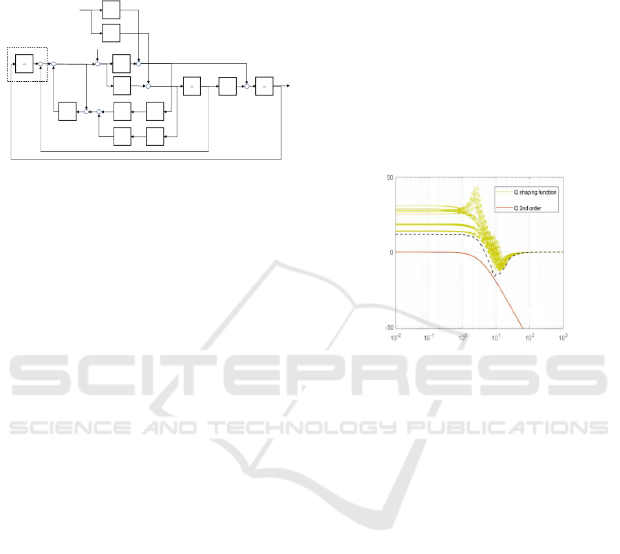
Figure 5 shows the overall block scheme,
and
are the transfer functions between the force and the
lateral velocity / angular velocity.
Figure 5: Block diagram under lateral force.
In order to facilitate the stability analysis of the system,
the path-following controller defined in Equation (1)
and the lateral error relationship have been linearized:
(12)
(13)
By analysing the block scheme, the transfer function
between the lateral error and the external lateral force,
by setting to zero its static gain and considering:
(14)
the following formulas can be retrieved:
(15)
As it can be observed from Equation (15), not only the
optimal gains depend solely on the nominal model, but
they are also independent from both the point of
application of the force (
), and its magnitude. This
result is of particular interest for a practical
implementation of the algorithm, since lateral forces
are hardly ever measured in a real scenario.
3.3 Low Pass Filter Choice
The choice of a proper low pass filter Q is an important
task in DoB design. As a matter of fact, this
component is responsible of reducing the negative
effects of high frequency measurement noises and
ensuring the robust stability of the closed-loop system
against unknown model parameters (Nguyen et al,
2014). To this scope, Q has been designed by
considering the model uncertainties as multiplicative
terms, represented in Equation (16) as:
(16)
By exploiting the small gain theorem, the following
sufficient condition, that guarantees the input/output
stability of the system, has been retrieved:
(17)
thus leading to:
(18)
This condition has finally been used to design the low-
pass filter.
Figure 6: Frequency constraints imposed on the low-pass
filter.
Figure 6 shows the shaping functions, represented by
Equation (18), evaluated from a set of plausible
parameters, and a possible filter’s candidate.
A second order low-pass filter with a cut-off
frequency of 0.53 Hz has been chosen in order to meet
the above constraint in the worst-case scenario:
4 SIMULATION RESULTS
In order to test our proposed control architecture, a
dynamic model of the tractor has been realized using
the MATLAB/Simulink environment. This model
has been developed according to (MathWorks,
2018) and (Narby, 2006), and it includes the
dynamics of the vehicle body, the dynamics of the
wheels, and also the tire relaxation model (Werner,
2015) needed to compute longitudinal and lateral
forces. We develop the model as time-continuous
model. Table 1 shows all the relevant parameters of
the tractor model.
-
-
+
+
+
+
+
+
-
+
+
+
+
Linearized controller
Magnitude [dB]
Frequency [rad/ s]
Bode Diagram
ICINCO 2019 - 16th International Conference on Informatics in Control, Automation and Robotics
254
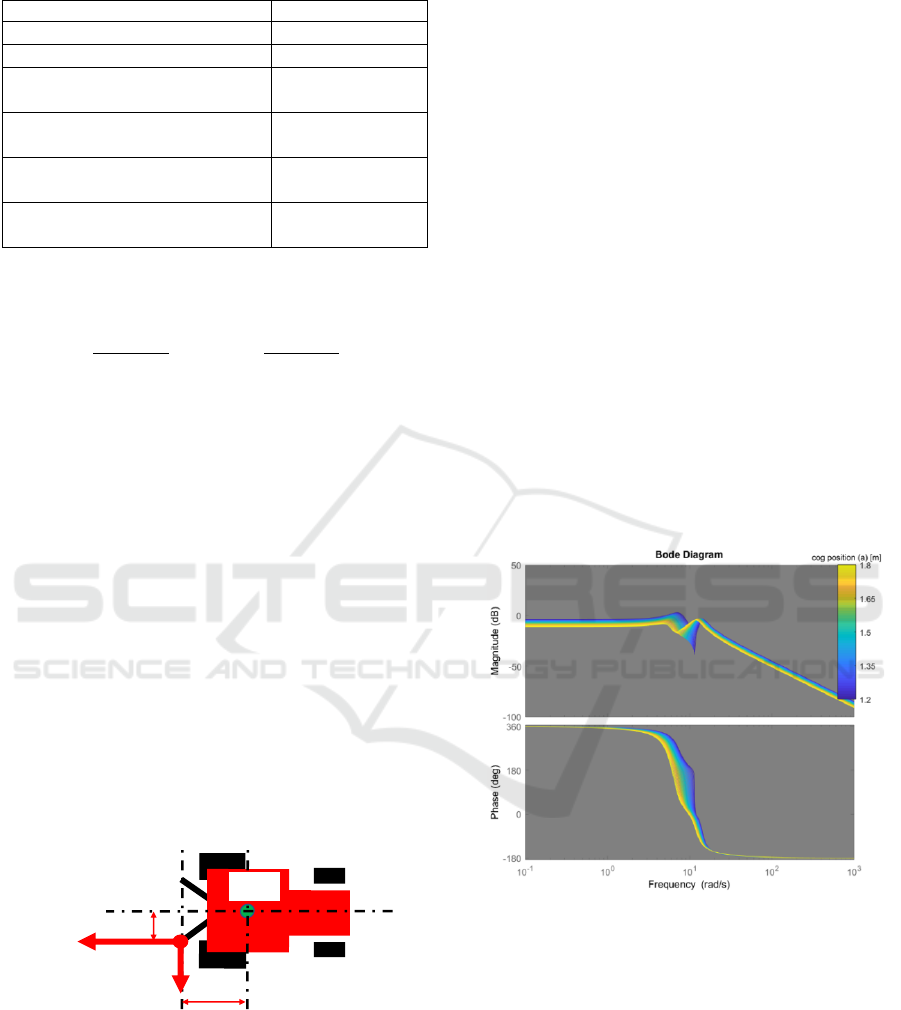
Table 1: Simulation parameters.
Parameter
Value
Vehicle mass ()
4203.6 kg
Moment of Inertia (
2416.0 kgm2
Normarized lateral front tire
stiffness (
4.18 1/rad
Normarized lateral real tire
stiffness (
1.5469 1/rad
Distance between CoG and
front tire axle()
1.67 m
Distance between CoG and
rear tire axle()
0.73 m
In addition, the tire cornering force is calculated as
follows:
(19)
where represents the gravity acceleration.
The effectiveness of our control algorithm has been
proved by considering three different simulation
scenarios: plowing, moving on inclined field and
moving in presence of significant sensor noise.
During plowing operations, the implement pulls the
tractor and its asymmetrical structure exerts a lateral
force on the vehicle, as it is shown in Figure 8.
In order to simulate the effect of the external forces
exerted by the implement, load data measured during
previous experiments have been used as reference.
For the sake of completeness, a load cell was installed
on the implement’s attachment and forces were
acquired during working.
Given the fact that agricultural tractors usually work
at constant speed, we considered the vehicle moving
at 3.00 km/h on a straight path with a look ahead
distance of 4.00 m. Then, we input the external force
to the tractor as a step disturbance.
Figure 7: Plowing simulation.
The external force is activated at 30.00 sec from the
simulation start. The force value was set to 23000.00N
for longitudinal direction, 2000.00 N for lateral
direction. We here provide the results of three
different simulations. During the first one, the tractor
is controlled by the path-following algorithm
introduced in Section II. During the second one, the
DOB discussed in Section III is introduced. CoG
position is its correct nominal position ( =1.67 m,
m), and the optimal gains are computed
according to Equations (15), under the 3.00 km/h
velocity constraint, leading to the following values:
Finally, during the third simulation, the DOB is
implemented by choosing a different nominal model
with respect to the real system. As a matter of fact, the
main property of DOB is the capability to force the
system to behave like the nominal model. For this
reason, if
and
are chosen properly it’s possible
to improve the dynamic performances of the closed-
loop system. With such choice particular attention
should be put into the stability analysis, since the
mismatches between the nominal model and the real
system will be much bigger.
Figure 8 (Figure 9) shows the Bode diagram of the
transfer function between the steering angle and the
lateral velocity
(angular velocity ) with respect
to different CoG position values. A bigger bandwidth
is achieved for smaller values of .
Figure 8: Bode diagram from to
with respect to CoG.
In order to speed up the system response, the nominal
CoG position has been chosen closer to the front
wheels (a = 0.1 m, b = 2.3 m). In this case, DOB gains
are calculated as follows:
The I/O stability is guaranteed by Equation (18) as it
is shown by Figure 10.
Figure 11 shows the lateral errors corresponding to
the three simulations. In absence of DOB, the
controller is not able to reject the disturbance
CoG
0.2m
1.73m
Longitudinal
Force
Lateral
Force
Disturbance Observer for Path-following Control of Autonomous Agricultural Vehicles
255
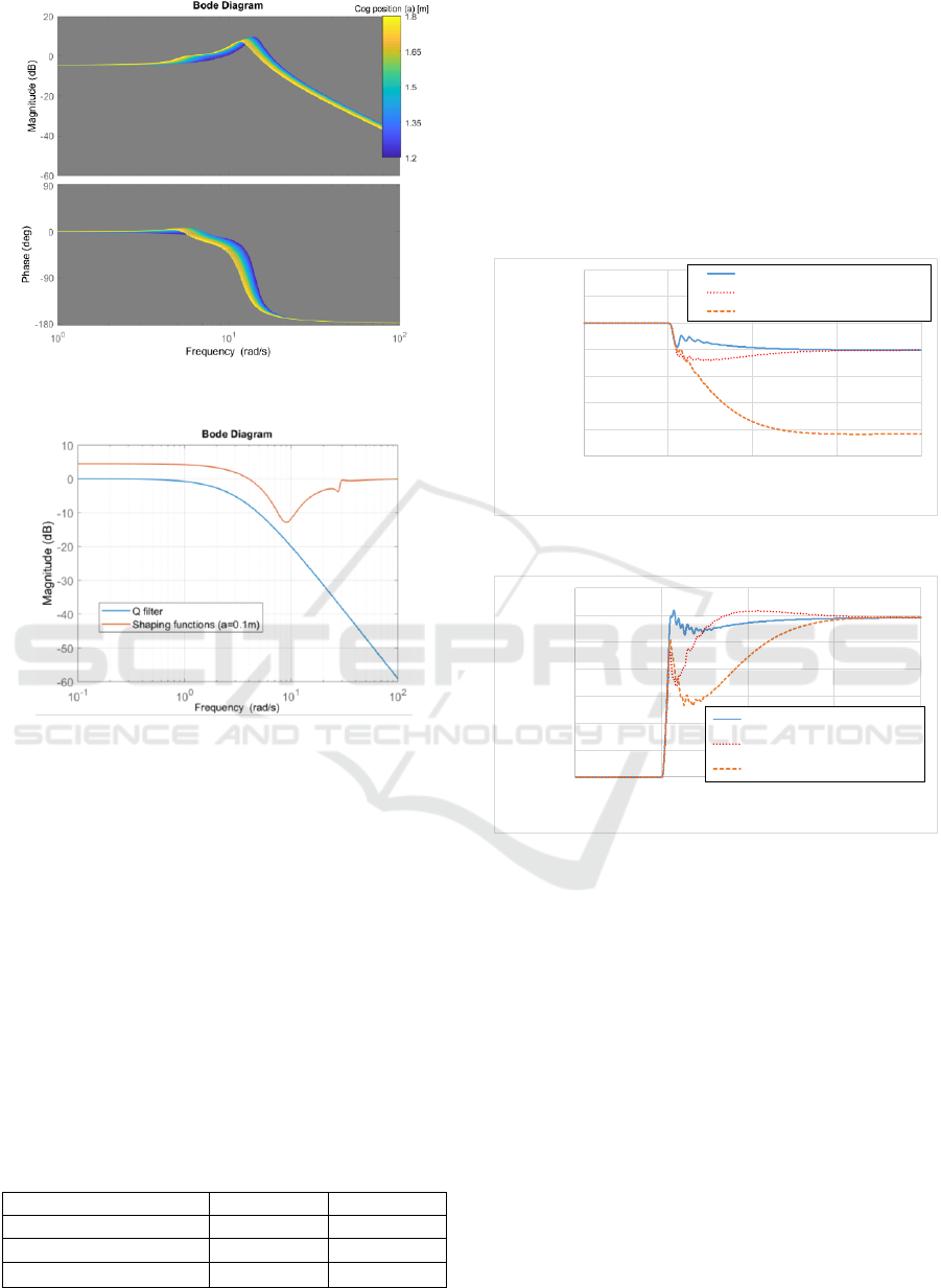
Figure 9: Bode diagram from to with respect to CoG.
Figure 10: Frequency constraints imposed on the low-pass
filter by choosing .
originating from the external force. As a result, the
lateral error rapidly increases and, more importantly,
the steady-state lateral error at the end of the transient
is not null. On the other hand, the controller endowed
with the DOB is able to reject the external force as
disturbance and to limit the lateral error. Moreover,
by setting a = 0.1 the transient response is improved,
but in the end, it converges to the same steady-state
value as the DOB using the correct nominal model.
To further prove the superior performance of our
approach, Table 2 shows the comparison among the
three control architectures in terms of Root Mean
Square Error (RMSE) and maximum error with
respect to the predefined path.
Table 2: Simulation Results about lateral error.
Controller
RMSE
Maximum
Path-Following
5.17 cm
8.34 cm
Nominal DOB-based
1.59 cm
2.78 cm
Modified DOB-based
1.29 cm
2.02 cm
Finally, Figure 12 shows the heading angle with
respect to the predefined path direction. Since we just
control the steering angle, all the controllers reach a
non-zero heading angle under the action of the
external force. That said, once again the two
controllers endowed with DOB (especially the one
characterized by a = 0.1) demonstrate superior
performance in terms of convergence time of the
heading angle with respect to the default path-
tracking controller.
Figure 11: Lateral error of plowing scenario.
Figure 12: Heading angle of plowing scenario.
Moving to the second simulation scenario, we here
consider the tractor moving on inclined ground. To
properly simulate the effect of gravity on the inclined
ground, a constant lateral force of acting on the CoG
is considered. More in depth, the force value was set
to 7000.00 N, since this value corresponds to the
lateral component of the gravity force of the simulated
tractor moving on a 10.00 degrees inclined field. Once
again, the external force acts like a step disturbance
that is activated at 30.00 sec from simulation start. Not
differently from the previous scenario, we here
consider the results of three different simulations:
path-following control, nominal DOB-based control
and modified DOB-based control. Figure 13 shows
the lateral errors corresponding to the three
simulations.
-0.1
-0.08
-0.06
-0.04
-0.02
0
0.02
0.04
20 30 40 50 60
Lateral error [m]
Time [sec]
Modified DOB-based control
Nominal DOB-based control
Path-Following control
0
0.2
0.4
0.6
0.8
1
1.2
1.4
20 30 40 50 60
Heading angle [deg]
Time [sec]
Modified DOB-based control
Nominal DOB-based control
Path-Following control
ICINCO 2019 - 16th International Conference on Informatics in Control, Automation and Robotics
256
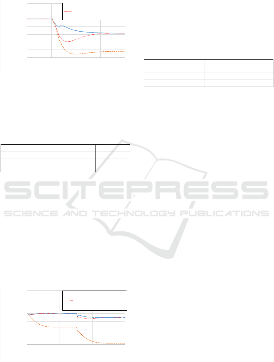
Figure 13: Lateral error of inclined scenario.
As far as RMSE and maximum error are concerned,
Table 3 shows the comparison among the three
controllers, further proving that our proposed
architecture guarantees a significantly lower error
with respect to the default path-following control.
Table 3: Simulation Results about lateral error.
Controller
RMSE
Maximum
Path-Following
11.44 cm
18.17 cm
Nominal DOB-based
6.10 cm
11.74 cm
Modified DOB-based
4.42 cm
7.37 cm
Finally, in the third simulation scenario we consider
the motion in presence of significant sensor noise. In
order to emulate this condition, we modify yaw rate
and steering angle measurements. As far as the
steering angle is concerned, the real value was edited
by adding a random white noise with 1.00 degree off-
set and amplitude equal to 10% of the signal
excursion. On the other hand, as far as the yaw-rate is
regarded, the amplitude of the additive noise is equal
to 1.00 degree/sec. The external force action is
simulated in the same way as the plowing scenario
and the simulation is repeated three times to collect
the outputs of the three different control strategies.
Figure 14 shows the lateral errors corresponding to
the three simulations.
Figure 14: Lateral error of sensor noise scenario.
Clearly, in this scenario the default path-following
controller is not able to counteract the effects of the
steering offset, while the two DOB-based controllers
successfully compensate it. Finally, Table 4 shows
the comparison of the three control algorithms in
terms of RMSE and maximum error.
Table 4: Simulation Results about lateral error.
Controller
RMSE
Maximum
Path-Following
10.92 cm
15.32 cm
Nominal DOB-based
1.61 cm
2.81 cm
Modified DOB-based
1.31 cm
2.15 cm
Given the fact that the typical desired motion accuracy
is 5.00 cm (RMSE) and 10.00 cm (maximum), we can
state that the proposed control algorithm is completely
compliant with the imposed requirements.
5 CONCLUSIONS
In this paper, we propose a DOB-based path-
following control algorithm able to improve the
accuracy of an autonomous agricultural tractor in
terms of lateral error with respect to a pre-defined
path. The DOB was designed on the basis of the
single-track vehicle model. The effectiveness of the
proposed control architecture was tested in a
simulation environment, considering three different
scenarios: plowing, moving on inclined field and
moving in presence of significant sensor noise.
Results show that the proposed controller is able to
reduce lateral error to 5 cm (RMSE) and 10 cm
(maximum), among all the considered scenarios.
As far as future developments are concerned, we’ll try
to apply the same DOB-based control architecture to
tracked vehicles, such as combine harvesters. Due to
the fact that the kinematics of tracked vehicles does
not allow to directly express the transfer function
between the lateral velocity and the angular velocity
of the vehicle, a different modelling approach will be
considered, like for instance the one proposed in
(Morita et al, 2018). On the other hands, an adaptive
control scheme for the implementation of a DOB on
tracked vehicles will also be considered. One possible
approach regarding tracked mobile robot is proposed
in (Hiramatsu et al, 2019). Finally, we will integrate
these experience to the real agricultural vehicles.
REFERENCES
Ball, D., Ross, P., English, A., Milani, P., Richards, D.,
Bate, A., Upcraft, B., Wyeth, G., Corke, P., 2017. Farm
-0.2
-0.16
-0.12
-0.08
-0.04
0
0.04
0.08
20 30 40 50 60
Lateral error [m]
Time [sec]
Modified DOB-based control
Nominal DOB-based control
Path-Following control
-0.16
-0.12
-0.08
-0.04
0
0.04
0.08
0.12
0 20 40 60
Lateral error [m]
Time [sec]
Modified DOB-based control
Nominal DOB-based control
Path-Following control
Disturbance Observer for Path-following Control of Autonomous Agricultural Vehicles
257

workers of the future. In IEEEE Robotics & Automation
Magazine.
Blackmore, S., 2009. New concepts in agricultural
automation. In HGCA conference.
Fang, H., Fan, R., Thuilot, B., Martinet, P., 2005. Trajectory
tracking control of farm vehicles in presence of sliding,
In IEEE/RSJ International conference on Intelligent
Robots and Systems.
Hiramatsu, T., Morita, S., Pencelli, M., Niccolini, M.,
Ragaglia, M., Argiolas, A., 2019. Path-Tracking
controller for tracked mobile robot on rough terrain, In
International conference on field and service robotics.
Huang, D., Hai, J., 2015. Trajectory tracking control of
wheeled mobile robots based on disturbance observer,
In IEEE Chinese Automation Congress.
Hyungbo, S., Gyunghoon, P., Youngjun, J., Juhoon, B.,
Nam Hoon, J., 2016. Yet another tutorial of disturbance
observer: robust stabilization and recovery of nominal
performance. In Control theory and technology. South
China University of technology and academy of
mathematics and systems science, vol. 14.
Lenain, R., Thuilot, B., Cariou, C., Martinet, P., 2004.
Adaptive and predictive nonlinear control for sliding
vehicle guidance, In IEEE/RSJ International
conference on Intelligence Robots and Systems.
MathWorks, 2018 Modeling a vehicle dynamics system,
retrieved February 7, 2019 from
https://jp.mathworks.com/help/ident/examples/modeli
ng-a-vehicle-dynamics-system.html?lang=en.
Morita, S., Hiramatsu, T., Niccolini, M., Argiolas, A.,
Ragaglia, M., 2018. Kinematic track modelling for fast
multiple body dynamics simulation of tracked vehicle
robot, In The 24th International Conference on
Methods and Models in Automation and Robotics.
Narby, E., 2006. Modeling and estimation of dynamics tire
properties, In examensarbete, Department of Electrical
Engineering Linköpings tekniska högskola Linköpings
universitet.
Nguyen, B., M., Fujimoto, H., Hori Y., 2014. Yaw angle
control for autonomous vehicle using Kalman filter
based disturbance observer. In SAEJ. EVTeC and APE
Japan.
Noguchi, N., Barawid Jr, O, C., 2011. Robot farming
system using multiple robot tractors in Japan
agriculture. In 18
th
IFAC world congress Milano.
Pentzer, J., Brennan, S., Reichard, K., 2014. Model-based
Prediction of Skid-steer Robot Kinematics Using
Online Estimation of Track Instantaneous Centers of
Rotation, In Journal of Field Robotics.
Rathgeber, C., Winkler, F., Odenthal, D., Muller, S., 2015.
Disturbance observer for lateral trajectory tracking
control for autonomous and cooperative driving. In
International journal of mechanics and mechatronics
engineering vol. 9.
Samuel, M., Hussein, M., Mohamad, B., Lucky, W., 2016.
A review of some pure-pursuit based path tracking
techniques for control of autonomous vehicles, In
International journal of computer applications.
Shalal, N., Low, T., McCarthy, C., Hancock, N., 2013. A
review of autonomous navigation systems in
agricultural environments, In SEAg 2013.
Taghia, J., Katupitiya, J., 2013. A sliding mode controller
with disturbance observer for a farm vehicle operating
in the presence of wheel slip. In IEEE/ASME
international conference on advanced intelligent
mechatronics.
Wen-Hua, C., Jun, Y., Lei, G., Shihua, L., 2016.
Disturbance-observer-based control and related
methods – An overview. In IEEE Transl. Industrial
electronics., vol. 63.
Werner, R., 2015. Centimeter-level accuracy path tracking
control of tractors and activity steered implements.
Ph.D. thesis, Technischen Universität Kaiserslautern
zur Verleihung des akademischen Grades.
Yu, S., Wang, J., Wang, Y., Chen, H., 2018. Disturbance
observer based control for four wheel steering vehicles
with model reference. In IEEE/CAA Journal of
Automatica Sinica,
ICINCO 2019 - 16th International Conference on Informatics in Control, Automation and Robotics
258
