
Microgrid Modeling Approaches for Information
and Energy Fluxes Management based on PSO
Li Qiao
1,2
, Rémy Vincent
2
, Mourad Ait-Ahmed
2
and Tang Tianhao
1
1
The Institute of Electric Drives and Control Systems, Shanghai Maritime Univ., Shanghai 201306, China
2
IREENA, Université de Nantes, Saint-Nazaire 44603, France
Keywords: Microgrid, Energy Management, PSO, MATLAB/SIMULINK.
Abstract: In order to improve the reliability, stability and economy of power supply of a microgrid, some fundamental
work on microgrid energy management method is carried out. Firstly, models of microgrid components under
steady state are established in MATLAB/SIMULINK. Secondly, an operation cost function of microgrid is
proposed, together with the constraint conditions. Then, in order to solve the energy management problem,
Particle Swarm Optimization (PSO) is declared by using m-files programming. The algorithm will be
explained in chart flow and pseudo code. Finally, a simulation scenario is designed to show the good
performance of this control method.
1 INTRODUCTION
As the global energy crisis and environmental
problems are becoming more serious, much attention
has been paid to renewable energy generation such as
wind power, solar power, etc. Safety stability
problems will be likely to occur if these power
resources are directly connected to the power grid. In
order to make full use of renewable energy generation,
the microgrid (MG) is generated in the field of
distributed generation. In general, a microgrid can be
defined as a combination of Distributed Energy
Resource (DER) units, which include Distributed
Generation (DG) units and Distributed Storage (DS)
units, and loads.
Microgrid is an independent and controllable
system and can achieve flexible conversion between
the grid-connected mode and the stand-alone (or
islanded) mode. A microgrid is able to switch
between these two modes. In the grid-connected
mode, the main grid can provide the compensation of
power short supply to the microgrid and take up the
excess power from the microgrid. A trade between the
microgrid and the main grid will be taken to maintain
the power balance. In the stand-alone mode of
operation, the power, whatever the real and reactive
power, should be kept in balance with the local loads
demands. A microgrid can be disconnected from the
main grid under two conditions: 1) Pre-planned
islanded operation: If any events in the main grid are
presented, such as long-time voltage dips or general
faults, among others, islanded operation must be
started; 2) Non-planned islanded operation: If there is
a blackout due to a disconnection of the main grid, the
microgrid should be able to detect this fact by using
proper algorithms.
If the microgrid can be managed effectively, the
reliability, stability and economy of power supply
will be improved effectively. The microgrid energy
management and strategy is one of the core problems
in microgrid research. A centralized Energy
Management System (EMS) for isolated microgrids
is proposed by Olivares, D.E, etc. Model predictive
control technique (MPC) is used to solve a multi-
stage MINLP problem iteratively. Fuzzy multi-
objective optimization model is set for a microgrid
taking the uncertainties of microgrid into account like
stochastic net load scenarios and uncontrollable
micro-sources. A system wide adaptive predictive
supervisory control (SWAPSC) approach, which
smooth the output of PV and wind generators under
intermittencies, maintains bus voltage by providing
dynamic reactive power support to the grid, and
reduces the total system losses while minimizing
degradation of battery life span, is proposed for a
microgrid with multiple renewable resources. The
energy management for microgird should also reach
some kind of goals or meet economic benefits. A
220
Qiao, L., Vincent, R., Ait-Ahmed, M. and Tianhao, T.
Microgrid Modeling Approaches for Information and Energy Fluxes Management based on PSO.
DOI: 10.5220/0007833002200227
In Proceedings of the 16th International Conference on Informatics in Control, Automation and Robotics (ICINCO 2019), pages 220-227
ISBN: 978-989-758-380-3
Copyright
c
2019 by SCITEPRESS – Science and Technology Publications, Lda. All rights reserved
social benefit cost made up of total generation cost,
maintenance cost of DGs and ESSs is given by Xiang,
Y. Another cost function composed of battery, new
power resources and exchange with grid is given by
Han, L. A more complex expression is shown by
Nikmehr, N, which includes four parts. The first part
is composed of the operation and maintenance cost of
generator, the second part only consist the installation
cost, the third part is the cost of money cost by energy
consumption and the forth part is the emission cost of
exhaust gas.
In this paper, an effectively way to management
microgrid will be discussed. The chapter 2 will list the
models of different microgrid components used in the
research. Chapter 3 will briefly give some
information about the system configuration. Chapter
4 is the operation design which includes the
description of objective functions and condition
constraints. The algorithms of PSO will also be talked
about in chapter 5. Chapter 6 is the simulation and
chapter 7 shows the future.
2 MODELING OF MICROGRIDS
Firstly, different parts of a typical microgrid
containing PV panel, wind turbine, battery, load,
diesel generator and corresponding converters are
modelled. There are two basic roles that have to be
mentioned:
All the components’ modelling is under steady
state
Power flow transitions are the only things this
paper cares
The first role steady-state means the dynamic
process is not taken into considering. During every
time step, the only thing that needs to be considered
is the initial value and final value. For example, if the
process of one certain time interval is a first-order
response, the actual curve used in this report just a
step. The second role means power output is the main
variable considering in energy management system.
Parameters like voltage, current are not considered.
The basic functions of different components are
like: PV panels are tending to generate power from
solar irradiation. Wind turbine will generate power
when the wind bellows. Battery storage system will
charge or discharge according to the power
difference. Diesel generator serves a main power
supply under all conditions.
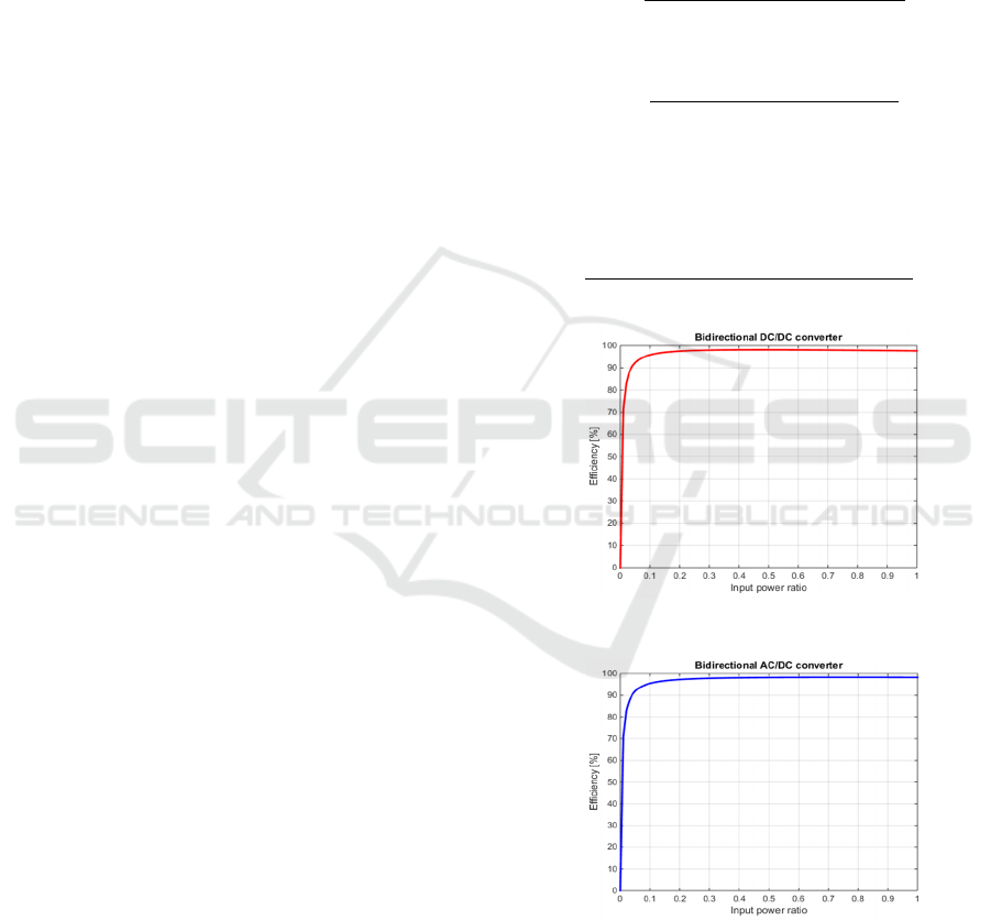
2.1 Electronic Converters
In the microgrid system, all the converters are
modelled as efficiency related to the input power and
converter rated power. The bidirectional DC/DC
converter efficiency the bidirectional AC/DC
converter efficiency can be formulated by the
Equation 1, 2:
100
0.007
1.00170.004
100%
(1)
100
0.018
1.0020.004
100%
(2)
Where u is the input power ratio, defined by
Equation 3:
(3)
Figure 1: DC/DC efficiency curve.
Figure 2: AC/DC efficiency curve.
Figure 1 and 2 shows the efficiency for
bidirectional DC/DC converter and bidirectional
AC/DC converter. It can be seen that the efficiency of
all these converters are nearly 98%. So if necessary,
Microgrid Modeling Approaches for Information and Energy Fluxes Management based on PSO
221

the value of efficiency may be taken as 98% in the
following work.
2.2 Solar Photovoltaic
A PV panel can be modelled in two ways: precise
model and simple model. Compared to the precise
one, the output of simplified PV model has
connection with the panel surface, the ambient
temperature, the solar irradiation and data from the
manufacture. The power output of PV is considered
at MPPT output, given by Equation 4:
∙∙
(4)
Where
is the output power of PV panel, is
the surface of a PV panel and is the real solar
irradiation received by PV panel.
is the power
transfer efficiency which is given by:
∙1
(5)
is the PV panel efficiency given by the
producer. is the temperature coefficient, usually
taken as 0.0045.
is the reference temperature.
Cell temperature
is deduced from ambient
temperature and solar irradiation in Equation 6:
∙
(6)
is the ambient temperature.
and
are ambient temperature and solar irradiation under
Nominal Operating Cell Temperature (NOCT)
conditions, with 20 ambient temperature and
800/
solar irradiation.
is the nominal
operating cell temperature.
2.3 Battery Storage System
For the battery, a lead-acid one with CIEMAT model
may be used. The most important parameter state of
charge (SOC) versus time can be described by:
∙
∙
3600∙
∙
(7)
∙
3600∙
∙
∙
(8)
Where
is the charging efficiency equals to
0.85, taking as the round-trip efficiency provided by
manufacture, and
is the discharging efficiency
equals to 1.
is the nominal capacity of the battery
and the
is the nominal battery voltage. As this is a
power battery model, the current and voltage may not
be important. The constraint is normally described as:
(9)
Where
and
are the maximum
and minimum allowable storage capacity.
2.4 Wind Turbine
The relationship between wind speed and the output
power of wind turbine can be described with
piecewise function, such as quadratic piecewise
function, linear piecewise function. A cubic
piecewise function is implemented, shown in
Equation 10, and the curve can be shown in Figure 3.
0,
∙
,
,
0,
(10)
Figure 3: Typical wind turbine power curve.
Where :
is the output power of wind turbine;
is the real wind speed;
is the rated power of wind turbine;
is the cut-in wind speed;
is the cut-out wind speed;
is the rated wind speed.
2.5 Diesel Generator and Load
The diesel generator is modelled as a power source
without an upper limit but with a lower limit to meet
the basic power consumption in microgrid.
ICINCO 2019 - 16th International Conference on Informatics in Control, Automation and Robotics
222
The load is considered as power consumption
component, varying with time.
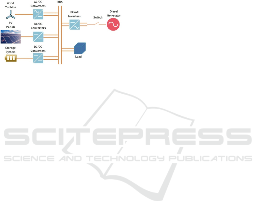
3 SYSTEM CONFIGURATION
Figure 4: System structure.
The typical structure of research object is shown in
Figure 4. The whole operation progress can be
explained as followed: the load demand power varies
with time. In order to keep the power balance on bus,
different components (PV, wind turbine, battery,
diesel generator) should provide power or absorb
power. So essence of this problem is power
distribution problem.
All the components are modelled in SIMULINK
environment. For the algorithm suitable for this
power distribution, a central controller using
MATLAB FUNCTION block is established.
The total simulation will be set under one day-24
hours, and sample time is set to 1 hour. To be specific,
it is a one-day-ahead plan, and the operation time
interval is 1 hour. The load data and weather data is
predicted and stored beforehand. So at each sample
time load power demand is detected, all the
components will send the power it can provide at this
certain time separately, according to the ambient
weather conditions. This power information will be
sent to the central controller, together with the load
demand. Then the central controller will decided the
actual power that each component needs to provide.
A rule-based energy management strategy is
firstly put forward. This method is simple and it
comes from human experience. The central controller
will ask PV, wind turbine, battery and diesel
generator in sequence for power supply. The
distributed power resources will give out power
according to their maximum output power
corresponding to the weather. And if possible, the
new energy resources will charge the battery if there
is abundant energy. Compared with this human-
experience-based algorithm, an optimal distribution
method using PSO will be discussed below.
4 OPERATION DESIGN
Economic optimization operation refers to the
comprehensive consideration of system economic,
environmental and technical benefits under the
premise of meeting system power balance and various
safe operation constraints, and optimizes the output
of each output unit in the distribution network.
4.1 Cost Function
The main objective of energy management is to
minimize the total cost of microgrid. The cost
function can be described as:
(11)
is the total cost of microgrid, which can be
divided into two parts: economic cost
and
environmental cost
.
The economic cost
is described in Equation
12.
(12)
∙
(13)
Where:
is the number of microgrids units;
is the power output of every unit;
is the fuel cost of every unit;
is the maintenance and operation cost of
each unit, which is given by Equation 13;
is the coefficient of maintenance and
operation of each unit.
When the microgrid is operating, there are some
pollutants such as CO2. Taken the environmental
benefit into consideration, the pollutants are
converting into a certain proportion, which is the
environmental cost. The environmental cost
is
defined in Equation 14.
∙
∙
(14)
Where :
Is the convert coefficient of pollutants;
is emission of unit product.
Microgrid Modeling Approaches for Information and Energy Fluxes Management based on PSO
223

4.2 Constraint Conditions
In order to reach a certain result, some constraints
must be added while solving the operation problem.
Power balance constraints
(15)
Where:
is the power demand from load;
is the output power of diesel generator;
is the output power of photovoltaic panels;
is the output power of wind turbine;
is the power exchange with battery.
PV constraints
0
,
(16)
,
represents the maximum power output of
PV panels under a certain weather condition
(temperature and solar irradiation), which is usually
considered as MPPT points. The real power output is
smaller than the value, but bigger than zero.
Wind turbine constraints
0
,
(17)
,
represents the maximum power output of
wind turbine under a certain weather condition (wind
speed). The real power output is smaller than the
value, but bigger than zero.
Diesel generator constraints
,
(18)
The output power of diesel generator must have a
minimum output in order to meet the basic load
demand.
Battery constraints
(19)
,
,
(20)
For a battery, the SOC should be restricted with a
suitable range. The power exchange
with
other components during a certain sample time should
also be limited.
5 OPTIMIZATION ALGORITHM
The operation design in previous chapter can be
concluded in such a form:
..
mi
n
0
0
(21)
Where:
is the objective function;
are the equality constraints;
are inequality constraints.
To solve such a nonlinear optimization problem,
traditional optimization methods may not find the
best result. Compared with other intelligent
algorithm, Particle Swarm Optimization (PSO) is
simple without too many parameters. Put forward by
Eberhart and Kennedy in 1995, PSO serves as an
effective method of optimization and has been widely
applied in various fields. It is the ideological source
of feeding the flock in the process embodied in the
collective wisdom.
5.1 Introduction to PSO
In short, PSO algorithm is to simulate the feeding
behavior of birds. Each bird is considered as a
particle. All of the particles have fitness values which
are evaluated by the fitness function to be optimized,
and have velocities which direct the flying of the
particles.
The basic procedure of PSO algorithm is shown
in Figure 5. PSO is initialized with a group of random
particles (solutions) and the searches for optima by
update generations. During every iteration, each
particle is updated by following two ‘best’ values.
The first one is the best solution (fitness) it has
achieved so far, and this fitness value is also stored.)
This value is called pbest. Another ‘best’ value that is
tracked by the particle swarm optimizer is the best
value, obtained so far by any particle in the
population. This best value is a global best and called
gbest.
After finding the two best values, the particle
updates its velocity and positions with Equation 22
and 23.
1
∙
∙
∙
∙
∙
(22)
ICINCO 2019 - 16th International Conference on Informatics in Control, Automation and Robotics
224
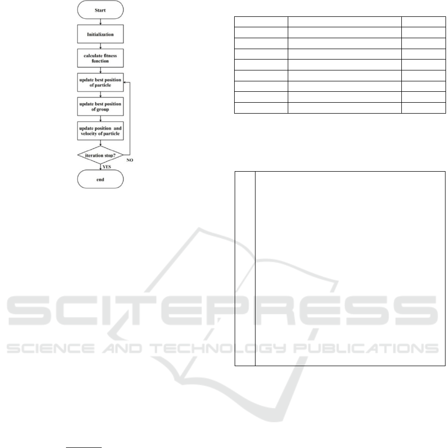
Figure 5: PSO algorithm chart flow.
1
1
(23)
Equation 22 is the formula for velocity updating,
and Equation 23 is the formula for position updating.
5.2 Modifications on PSO
However, due to the complexity of problem, the basic
method cannot be applied directly. It has to be
mentioned that some modifications are made to meet
this problem.
Simulation time is 24 seconds to represent 24
hours operating condition. The sample time is
1 hour which is using 1 second actually. So the
optimization algorithm is put in the outside
loop, which means the algorithm will be run 24
times, so that at each sample time an optimal
result will reach.
100%
(24)
As this is a multi-objective problem, after the
traditional PSO is completed, a ‘Pareto set’ will
appear. It means there are many optimal
answers COUPLED. So, after the ‘Pareto set’
is reached, it has to be filtered to require the
most wanted answer. The filtering method can
be described in Equation 24. The efficiency
should be as bigger as possible. When is
bigger, it means PV and wind turbine provides
more power, as a result, this answer is more
environmentally friendly.
The specific parameters of PSO are shown in
Table 1.
Table 1: Parameters for PSO.
Variables Explanations Values
N Number of particles 50
W_max Maximum inertia weight 1.05
W_min Minimum inertia weight 0.1
C1 Personal confidence factor 2
C2 Swarm confidence factor 2
MaxIter Number of iteration 100
v_max Maximum velocity 1.05
v_max Minimum velocity -1.05
5.3 Pseudocode Description
The pseudocode of PSO is shown below.
1
2
3
4
5
6
7
8
9
10
11
12
13
14
15
Read the power information from components.
External loop for 24 hours {
Initializing position, velocity, fitness function
and Pareto set.
Calculating fitness function initially.
Firstly filtering of Pareto set.
Inner loop for iteration {
Updating velocity and position.
Calculating fitness function.
Updating pbest (best position of particles).
Combining the previous Pareto set an
d
pbest in a new set.
Filtering new set.
} End for iteration.
Final Filtering and reserve the answer.
} End for
External loop
Plot
6 SIMULATION AND RESULTS
In this part, a total simulation will be estimated.
Firstly, the predicted weather data used are shown
from Figure 6 to Figure 8. With these figures, the
maximum output power under such ambient
condition will be calculated using the steady state
models from chapter 2.
Then a comparison between two strategies is
shown in Figure 9 and Figure 10. In the two figures,
the bar graph is the output power of a certain
resources and the height of bar determines the
quantity of power. The red line with star symbol is the
predicted load demand. It can be seen that the
algebraic sum of every bar-the power resources,
equals to the load demand, which the power balance
is met. It has to be mentioned that when the bar of
battery is negative, it means the battery is under
charge state, or under discharge state when positive.
Microgrid Modeling Approaches for Information and Energy Fluxes Management based on PSO
225
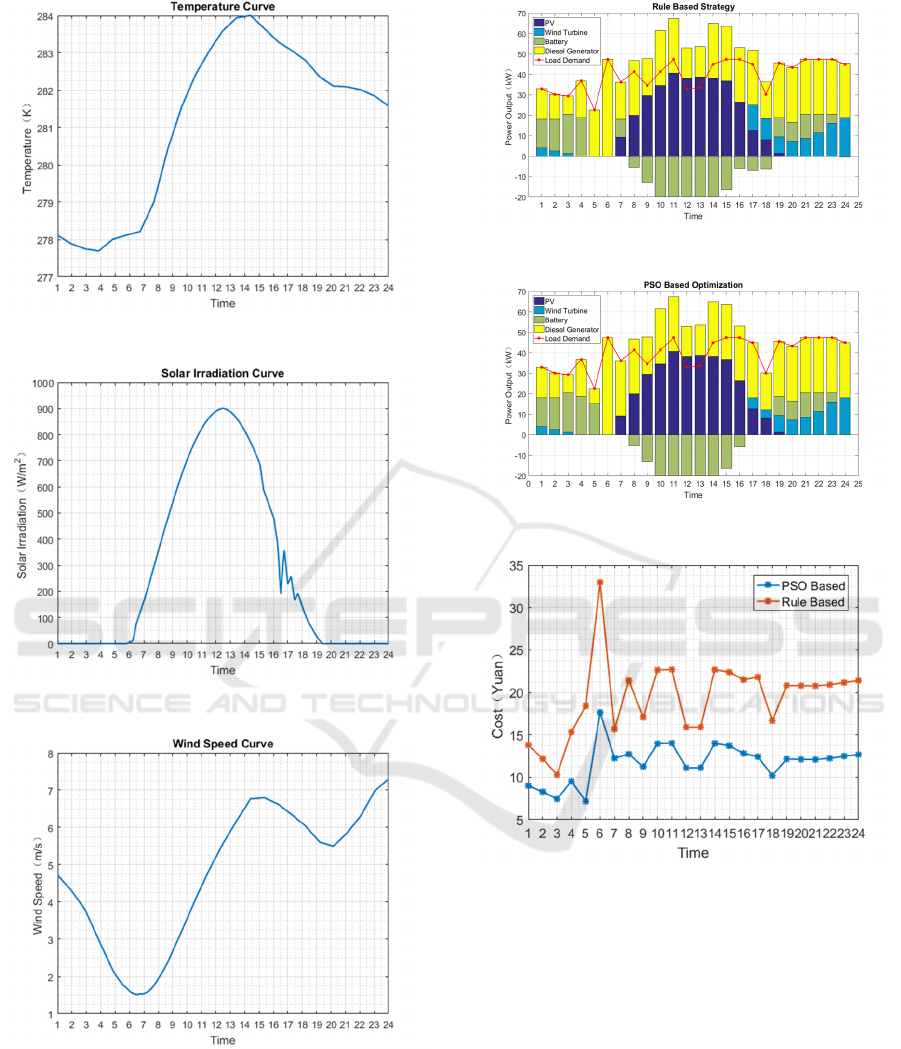
Figure 6: Temperature curve.
Figure 7: Solar irradiation curve.
Figure 8: Wind speed curve.
By calculating the cost function of two strategies,
shown in Figure 11, it can be seen that the cost using
PSO optimization is smaller than the human-
experienced-based strategy. The superiority of PSO
has been embodied.
Figure 9: Rule based strategy.
Figure 10: PSO based strategy.
Figure 11: PSO algorithm chart flow.
7 CONCLUSION AND REMARKS
This paper makes effective energy management for
the whole microgrid based on the particle swam
optimization algorithm. In the optimization process,
the economic and environmental aspects are
considered comprehensively. A multi-objective is
carried out with the lowest cost including economic
cost and environmental cost, and the good
performance of PSO is verified by an example.
For future work, here are some significant points:
ICINCO 2019 - 16th International Conference on Informatics in Control, Automation and Robotics
226

Multi-agent system can be designed to describe
the controllers of each component.
The PSO may be combined with other
intelligent control method to reach a better
performance of program running.
ACKNOWLEDGEMENTS
This paper is supported by National Natural Science
Foundation of China (Grant No: 61673260).
REFERENCES
Olivares, D. E., Mehrizi-Sani, A., Etemadi, A. H.,
Cañizares, C. A., Iravani, R., Kazerani, M.,
Hajimiragha, A. H., Gomis-Bellmunt, O., Saeedifard,
M., Palma-Behnke, R. and Jiménez-Estévez, G. A.,
2014. Trends in microgrid control. IEEE Transactions
on smart grid, 5(4), pp.1905-1919.
Vasquez, J. C., Guerrero, J. M., Miret, J., Castilla, M. and
De Vicuna, L. G., 2010. Hierarchical control of
intelligent microgrids. IEEE Industrial Electronics
Magazine, 4(4), pp.23-29.
Olivares, D. E., Cañizares, C. A. and Kazerani, M., 2014. A
centralized energy management system for isolated
microgrids. IEEE Transactions on Smart Grid, 5(4),
pp.1864-1875.
Li, P., Xu, D., Zhou, Z., Lee, W. J. and Zhao, B., 2016.
Stochastic optimal operation of microgrid based on
chaotic binary particle swarm optimization. IEEE
Transactions on Smart Grid, 7(1), pp.66-73.
Han, J., Khushalani-Solanki, S., Solanki, J. and Liang, J.,
2015. Adaptive critic design-based dynamic stochastic
optimal control design for a microgrid with multiple
renewable resources. IEEE transactions on Smart Grid,
6(6), pp.2694-2703.
Xiang, Y., Liu, J. and Liu, Y., 2015. Robust energy
management of microgrid with uncertain renewable
generation and load. IEEE Transactions on Smart Grid,
7(2), pp.1034-1043.
Han, L., Jianhua, Z. and Rafique, S. F., 2017.
Implementation of battery management module for the
microgrid: a case study. Int. J. Smart Grid Clean Energy,
6(1), pp.11-20.
Nikmehr, N. and Najafi-Ravadanegh, S., 2015. Optimal
operation of distributed generations in micro-grids
under uncertainties in load and renewable power
generation using heuristic algorithm. IET Renewable
Power Generation, 9(8), pp.982-990.
Kakigano, H., Miura, Y., Ise, T., Van Roy, J. and Driesen,
J., 2012, November. Basic sensitivity analysis of
conversion losses in a DC microgrid. In 2012
International Conference on Renewable Energy
Research and Applications (ICRERA) (pp. 1-6). IEEE.
Diaf, S., Notton, G., Belhamel, M., Haddadi, M. and
Louche, A., 2008. Design and techno-economical
optimization for hybrid PV/wind system under various
meteorological conditions. Applied Energy, 85(10),
pp.968-987.
Bouabdallah, A., Olivier, J. C., Bourguet, S., Machmoum,
M. and Schaeffer, E., 2015. Safe sizing methodology
applied to a standalone photovoltaic system. Renewable
energy, 80, pp.266-274.
Zaibi, M., Champenois, G., Roboam, X., Belhadj, J. and
Sareni, B., 2018. Smart power management of a hybrid
photovoltaic/wind stand-alone system coupling battery
storage and hydraulic network. Mathematics and
Computers in Simulation, 146, pp.210-228.
Sechilariu, M., Wang, B. C., Locment, F. and Jouglet, A.,
2014. DC microgrid power flow optimization by multi-
layer supervision control. Design and experimental
validation. Energy conversion and management, 82,
pp.1-10.
Abbes, D., Martinez, A. and Champenois, G., 2014. Life
cycle cost, embodied energy and loss of power supply
probability for the optimal design of hybrid power
systems. Mathematics and Computers in Simulation, 98,
pp.46-62.
Microgrid Modeling Approaches for Information and Energy Fluxes Management based on PSO
227
