Enhancing Neural Network Prediction against Unknown Disturbances

with Neural Network Disturbance Observer

Maxime Pouilly-Cathelain

1,2

, Philippe Feyel

, Gilles Duc

and Guillaume Sandou

Safran Electronics & Defense, Massy, France

L2S, CentraleSup

elec, CNRS, Universit

e Paris-Sud, Universit

e Paris-Saclay, Gif-sur-Yvette, France

Keywords:

Neural Network, Prediction, Disturbance Observer.

Abstract:

Neural network prediction is a very challenging subject in the presence of disturbances. The difﬁculty comes

from the lack of knowledge about perturbation. Most papers related to prediction often omit disturbances but,

in a natural environment, a system is often subject to disturbances which could be external perturbations or also

small internal parameters variations caused, for instance, by the ageing of the system. The aim of this paper

is to realize a neural network predictor of a nonlinear system; for the predictor to be effective in the presence

of varying perturbations, we provide a neural network observer in order to reconstruct the disturbance and

compensate it, without any a priori knowledge. Once the disturbance is compensated, it is easier to realize

such a global neural network predictor. To reach this goal we model the system with a State-Space Neural

Network and use this model, completed with a disturbance model, in an Extended Kalman Filter.

1 INTRODUCTION

Most of controlled processes are very sensitive to dis-

turbances that may be of different natures; on the one

hand, they can model real external disturbances or,

on the other hand, internal parameter variations of

the system provided that they are small enough (Chen

et al., 2000). In this paper, we aim to model nonlin-

ear systems by using neural networks in order to get

a predictor. For instance, this predictor can be used

in a Model Predictive Control (Yu and Gomm, 2003),

being in that case initialized by the measure at each

time step following the so-called receding horizon

principle (Keviczky and Balas, 2006). Usually, for

the training task, the neural network used for predic-

tion purpose is a Feedforward Neural Network (FNN)

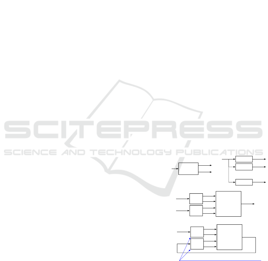
preceded by tapped delay lines (TDL, deﬁned in ﬁg-

ure 1). For the prediction task, the neural network is

then artiﬁcially looped into a Nonlinear AutoRegres-

sive eXogeneous model (NARX). This method, sum-

marized in ﬁgure 1, is similar to the one presented

in (Hagan et al., 1996) (Chapter 27) and has proved

its efﬁciency for different kinds of systems (Hed-

jar, 2013), (Diaconescu, 2008). This neural network

structure is preferred because it is easy to be trained

ofﬂine and online contrary to recursive structures as

shown in (Pascanu et al., 2013). Moreover, training

this structure online allows to learn small parameters

variations that can be modeled by small disturbances,

however we aim to deal with relatively high distur-

bances in this paper.

Tapped Delay

Line (TDL)

deﬁnition

TDL

: n

)

(=)

−n

−(n

+1)

−n

Learning task

(FNN)

TDL

(0 : n

)

TDL

(1 : n

)

mes

Prediction task

(NARX)

TDL

(0 : n

)

TDL

(1 : n

)

Initialized by previous measures at each time step

Figure 1: Neural network prediction using FNN/NARX

models.

However, using such a method leads to inaccurate

prediction results in the face of varying disturbance

proﬁles or parameter variations. Indeed, the neural

network is trained using some non-disturbed data or

some particular disturbance inputs. As a result, the

210

Pouilly-Cathelain, M., Feyel, P., Duc, G. and Sandou, G.

Enhancing Neural Network Prediction against Unknown Disturbances with Neural Network Disturbance Observer.

DOI: 10.5220/0007831102100219

In Proceedings of the 16th International Conference on Informatics in Control, Automation and Robotics (ICINCO 2019), pages 210-219

ISBN: 978-989-758-380-3

prediction remains well adapted to these particular sit-

uations, but some large prediction errors may arise in

other real-life situations characterized by other real-

istic disturbance proﬁles or system parameter varia-

tions. This statement will be shown with the example

at the end of the paper.

With the aim of improving the performance of the

predictor against unknown disturbances that can vary

or vanish, a natural idea is to estimate the current

disturbance. The observed perturbation will then be

used as a feedback compensator to make the system

less sensitive to disturbances. Some solutions have al-

ready been proposed in the literature. (Vatankhah and

Farrokhi, 2017) presents an observer based on a neu-

ral network inverse model to ﬁnd the inverse model

of the system with an ofﬂine identiﬁcation: it allows

to reconstruct the control signal and so to deduce the

perturbation. The main drawback of this method is

that it supposes that the perturbation signal is avail-

able during the training process. Moreover, the iden-

tiﬁcation of the static inverse neural network model is

not efﬁcient in case of parameter variations. (Talebi

et al., 2010) and (Lakhal et al., 2010) have devel-

oped an adaptive observer based on backpropagation

which is a well-known neural network learning algo-

rithm (Werbos, 1974). An idea could be to combine

this method with a disturbance observer. However the

steady state error, although bounded, does not asymp-

totically converge to zero and the disturbance may not

be well reconstructed.

In this study, the aim is to asymptotically

reconstruct the perturbation without any direct

measurement of the perturbation.

To improve the predictor performance for a plant

subject to a varying disturbance, the following three

steps methodology, summarized in ﬁgure 2, is pro-

posed in this paper:

• The plant is modelled as a State-Space Neural

Network (SSNN), ofﬂine trained without distur-

bances. This neural network structure has been

chosen because, contrary to the NARX structure,

it can be easily used as an observer.

• The state of the SSNN model is augmented

with the searched disturbance to be reconstructed.

Then, by using this new augmented model, an Ex-

tended Kalman Filter (EKF) reconstructs the aug-

mented state and thus the disturbance.

• The observed disturbance is ﬁnally used as a feed-

back compensator for the purpose of compensat-

ing the perturbation effect.

This paper is organized as follows. In section 2,

corresponding to the ﬁrst step of the methodology,

the structure of the neural network used to model the

plant and the associated training method is presented.

The second step is presented, in section 3 where the

EKF formulation is reminded and applied to a simple

example of SSNN. Finally, the compensator design

is the core of section 4. Numerical results to prove

the viability of the approach are given in section 5

and section 6 concludes and gives some forthcoming

works.

This study can easily be extended to MIMO (Multi

Input Multi Output) systems but, for simplicity of

equations and schemes, we will only present the

method for SISO (Single Input Single Output) sys-

tems. By the way, the example corresponds to a SIMO

system.

Ofﬂine training of

the SSNN model

without any

disturbance

Augmentation of

the SSNN state with

the disturbance Γ

and realization of

an EKF

Use of the

estimated

disturbance as a

feedback

compensator

Step 1

Section 2

Step 2

Section 3

Step 3

Section 4

Figure 2: Three steps proposed method.

2 STATE-SPACE NEURAL

NETWORK MODELING

2.1 State-Space Neural Network

(SSNN)

In order to be able to model any kind of nonlinear-

ity we have chosen to use a neural network (Hagan

et al., 1996) due to its ability to approximate any kind

of static function (Cybenko, 1989). Because of the

dynamical property of the considered system, it is re-

quired to use recurrent neural networks (RNN). It ex-

ists many different structures of recurrent neural net-

works, (De Jesus and Hagan, 2007) gives some exam-

ples. The SSNN structure (Figure 3) seems us more

suitable to be used in nonlinear observer techniques

such as extended Kalman ﬁlter. Some properties of

the SSNN structure can be found in (Zamarre

no and

Vega, 1998).

Enhancing Neural Network Prediction against Unknown Disturbances with Neural Network Disturbance Observer

211

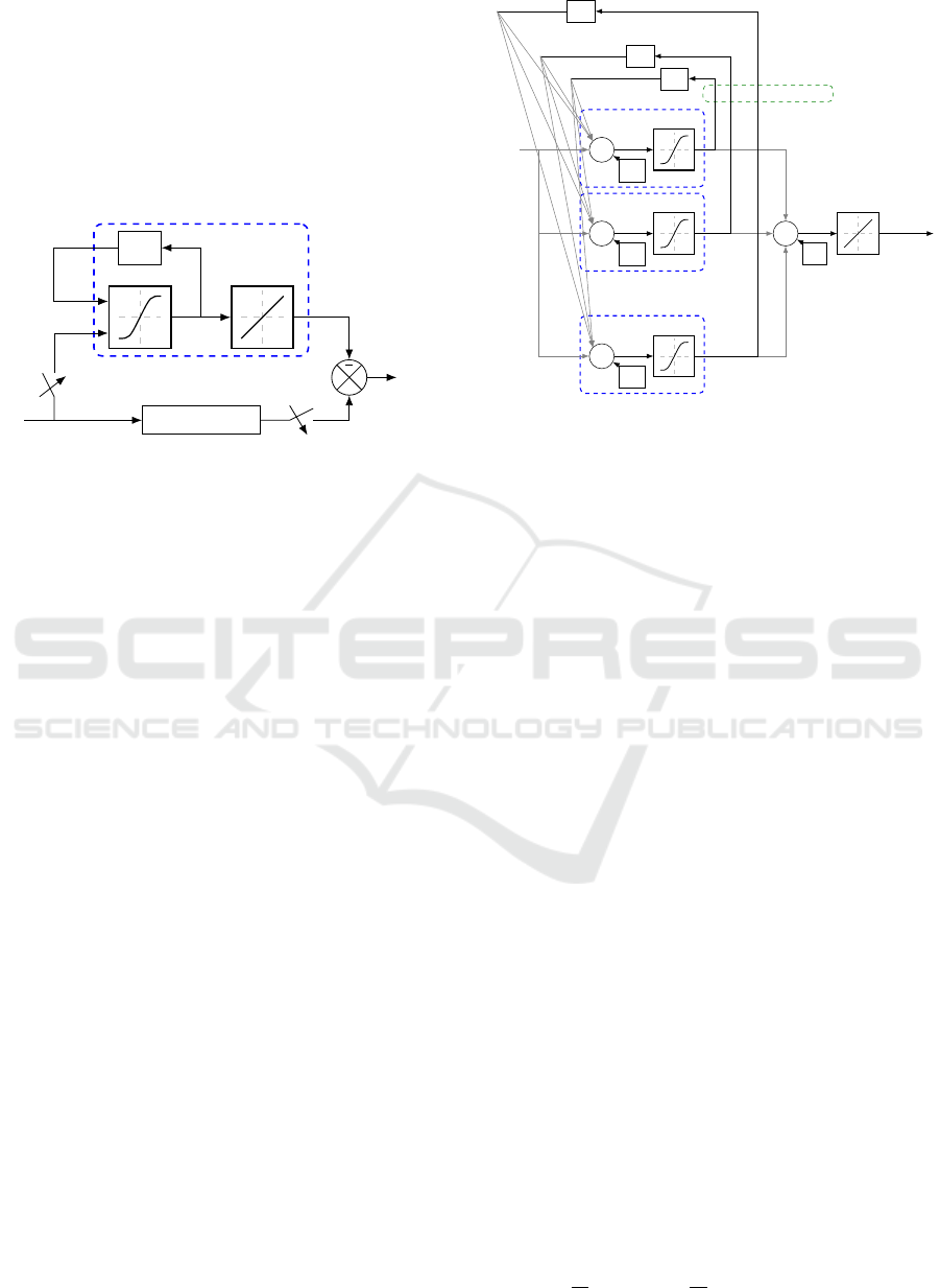
Figure 3 deﬁnes the following notation: u is the

input signal, T

is the sampling period, k the sampling

index, X the internal state vector of the SSNN, y

the

output of the SSNN, y the output of the plant, e the er-

ror between the plant and the model and z

−1

the delay

operator. The hidden layer has a nonlinear activation

function and the output layer has a linear activation

function.

SSNN

Plant

−1

u(t)

e[k]

[k]

X[k]

y(t)

y[k]

Figure 3: SSNN model of the plant.

The SSNN structure contains internal states that

model the dynamics of the system. The number of

neurons of the hidden layer, noted n, is equal to the

number of internal states. These states do not have

any physical meaning and n is a compromise between

accuracy of the model and complexity (essentially in

terms of computation time and memory needed for

the learning process). The SSNN is represented by:



X[k +1] = σ(W

h,u

u[k] +W

h,X

X[k] + B

)

[k] = W

X[k] + B

, (1)

where X ∈ R

n×1

is the internal state vector, W

h,u

∈

n×1

are the weights of the ﬁrst layer related to the

input u, W

h,X

∈ R

n×n

the weights of the ﬁrst layer re-

lated to the state X, B

∈ R

n×1

the bias of the ﬁrst

layer, W

∈ R

1×n

the weights of the ﬁnal layer, B

∈ R

the bias of the ﬁnal layer. The activation function of

the hidden layer σ is the sigmoid function deﬁned by:

σ(x) = 1/(1 + exp(−x)). (2)

This activation function has to be evaluated for

each component of the vector in (1). Equation (1)

is directly a state-space representation of a nonlinear

system. The identiﬁcation process (also named learn-

ing or training process) aims to determine the values

of W

h,u

, W

h,X

, B

, W

and B

Figure 4 shows the details of the internal SSNN

structure. We note B

= [b

,.. . ,b

]

Neuron 1

Neuron 2

Neuron n

−1

··· n states

u[k]

[k]

Figure 4: SSNN (grey arrows are weighted connections).

2.2 Training task of the State-Space

Neural Network

The identiﬁcation process is realized ofﬂine once for

all. All training data can be acquired with or with-

out disturbances. However, in the former case, the

estimated disturbance will not correspond to the real

one because the SSNN model will take into account

the disturbance included in the training data. For in-

stance, if the training set contains an additive input

disturbance Γ

train

and if we use the system in pres-

ence of another disturbance Γ

use

then the estimated

disturbance

Γ will be deﬁned by (3).

Γ = Γ

use

− Γ

train

. (3)

For clarity, we suppose in the sequel that the train-

ing data are obtained without disturbances.

Because the SSNN is a recurrent neural network,

classical learning algorithms such as Backpropaga-

tion [8] cannot be used. Many learning algorithms

have been developed to deal with recurrent neu-

ral networks such as Real Time Recurrent Learning

(RTRL) (Williams and Zipser, 1989), BackPropaga-

tion Through Time (BPTT) (Werbos, 1990) and De-

coupled Extended Kalman Filter (DEKF) (Haykin,

2004). The two main learning algorithms for RNN are

RTRL and BPTT which are both presented in (Hagan

et al., 1996). The RTRL, combined with the well-

known Levenberg-Marquardt (LM) method (Leven-

berg, 1944), (Marquardt, 1963), is used in this study.

These algorithms use the cost function deﬁned by (4).

∑

k=1

[k] =

∑

k=1

(y[k] − y

[k])

, (4)

ICINCO 2019 - 16th International Conference on Informatics in Control, Automation and Robotics

212

where n

is the number of samples.

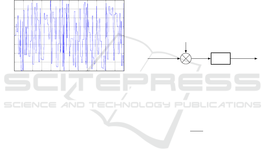
Usually, the input signal is chosen to be square

with random amplitudes and durations (between min-

imum and maximum values deﬁned by the user) in

order to stimulate the system for all possible conﬁg-

urations. For that purpose, it is supposed that bounds

on the admissible input amplitudes are known as well

as an order of magnitude of the system time response.

For instance, a possible input signal for a system with

input levels in the range [−2;2] and a time response

equals to 1s is presented in ﬁgure 5.

In the sequel, all inputs and outputs data have to

be normalized.

45 50 55 60

−2

−1.5

−1

−0.5

0.5

1.5

Time (s)

Amplitude

Input

Figure 5: Example of input signal.

RTRL is a deterministic algorithm but a starting

point is needed and randomly chosen. Thus, several

runs with different initializations can be done, hoping

the result to be closer to the global minimum. More-

over, in order to avoid overﬁtting (and so to improve

the prediction capacity with regard to different operat-

ing conditions) an early stopping has been performed

by using a validation set as proposed in (Sarle, 1995).

The data set is thus divided in three different sets: a

training set, a validation set and a test set. The train-

ing set is used to train the system, the validation set

is used for generalization purpose and the test set is

used to test the neural network at the end of the train-

ing. Finally, the stopping criterion consists in one of

these conditions:

• the maximum number of iterations has been

reached,

• the cost function has reached the minimum value

deﬁned by the user,

• the cost function evaluated with the validation set

has increased for n

consecutive times, where n

is an integer deﬁned by the user.

The reader can get more information about RTRL

and LM respectively in (Williams and Zipser, 1989)

and (Gavin, 2017). The training of RNN can be a

challenging task for some systems. (Pascanu et al.,

2013) presents some difﬁculties that can occur during

the training and some solutions to improve the learn-

ing.

3 STATE-SPACE NEURAL

NETWORK DISTURBANCE

OBSERVER

3.1 Disturbance Model

As shown in ﬁgure 6, we consider in this paper that

a disturbance is added at the input of the system. As

a reminder, this disturbance can model external per-

turbations or internal parameter variations providing

that, depending on the system, they are small enough.

Disturbance Γ

Plant

Command u

u + Γ

Output y

Figure 6: Disturbed plant.

3.2 Augmented State with Disturbance

A common method to estimate disturbances is to

complete the state with a new state Γ that represents

the disturbance by enforcing:

dΓ(t)

= 0, (5)

The new augmented state vector X

can now be

deﬁned from the model proposed in ﬁgure 6 in which

the plant is the SSNN and X

= (X

,Γ

)

. In discrete

time we get (6).











[k + 1] =







h,u

(u[k] +C

[k])

h,X

[k] + B



[k]





[k] = W

[k] + B

(6)

where C

= [0

1×n

1] and C

= [I

n×n

n×1

Given X

from (6), we can implement a state ob-

server that will estimate X

and thus Γ.

3.3 Extended Kalman Filter (EKF)

The system (6) can be observed by using many non-

linear observation methods such as sliding mode ob-

server (Alessandri, 2000), EKF (Terejanu, 2008),

Enhancing Neural Network Prediction against Unknown Disturbances with Neural Network Disturbance Observer

213

Unscented Kalman Filter (UKF) (Wan and Van

Der Merwe, 2000), high-gain observer (Bullinger and

Allg

ower, 1997) or extended Luenberger observer

(Grossman, 1999). The EKF, which is a nonlin-

ear derivation of the original Kalman ﬁlter (Kalman,

1960), is used in this paper, for its simplicity of im-

plementation even if tuning the weights may be some-

times difﬁcult. Considering a system deﬁned by:



[k + 1] = f (X

[k], u[k],w[k])

[k] = h(X

[k], v[k])

. (7)

w[k] and v[k] are two white Gaussian noises with re-

spective covariance matrices Q[k] and R[k] that can

be used as tuning weights for the ﬁlter. One iteration

of the Extended Kalman Filter is concerned with two

steps, the prediction and the update ones, where the

use of the “hat” notation denotes the estimated val-

ues.

• Prediction step:



[k | k − 1] = f (

[k − 1],u[k], 0)

P[k | k − 1] = F[k]P[k − 1]F

[k] + Q[k]

(8)

• Update step:











˜y

[k] = y[k] − h



[k | k − 1],0



S[k] = H[k]P[k | k − 1]H

[k] + R[k]

K[k] = P[k | k − 1]H

[k]S

−1

[k]

[k] = X

[k | k − 1] + K[k] ˜y

[k]

P[k] = (I − K[k]H[k])P[k | k − 1]

. (9)

Where F[k] =

∂ f

∂X



[k−1],u[k]

and H[k] =

∂h

∂X



[k|k−1]

F[k] and H[k] can be easily computed from (6) since

the sigmoid function is differentiable:

(1)

(x) =

dσ(x)

exp(−x)

(1 + exp(−x))

(10)

and h is a linear function in the considered case (see

(6)). For instance, F and G are given in section 3.4

for a 2-neurons SSNN.

As states of the SSNN have no physical meaning,

an accurate reconstruction of all states is not the pri-

ority. It is suggested to tune the ﬁlter to give more

importance to the disturbance, that is the last compo-

nent of X

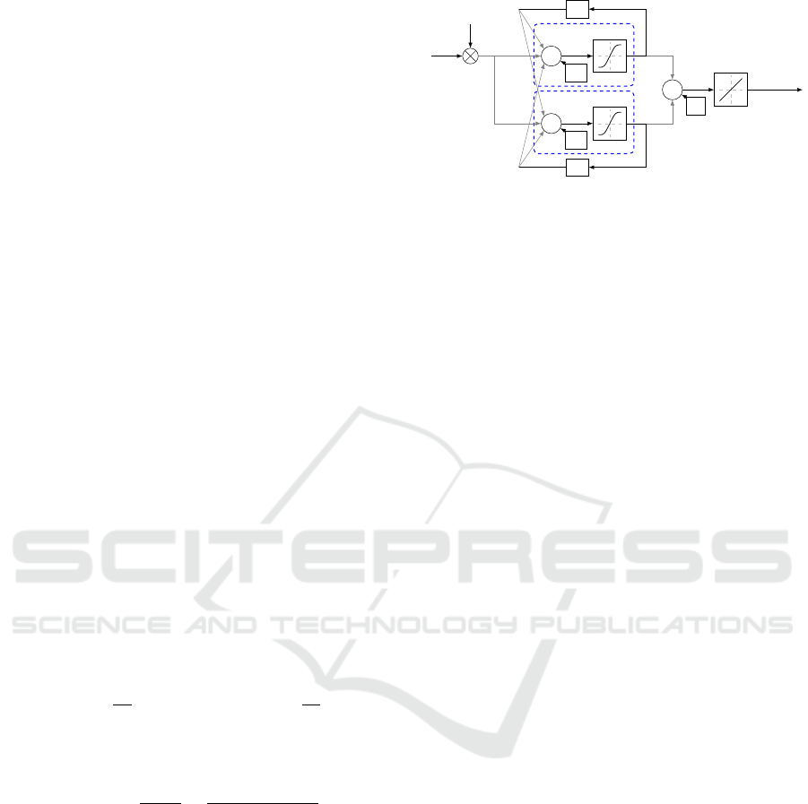
3.4 Example for a Two-neurons SSNN

To illustrate the computation of matrices F[k] and

H[k] of the Kalman ﬁlter, a model with two neurons

and dΓ(t)/dt = 0 is considered in this section.

Neuron 1

Neuron 2

−1

Γ[k]

u[k]

[k + 1]

1,1

2,1

1,2

2,2

Figure 7: Two neurons SSNN.

Figure 7 presents such a two-neurons SSNN.

We use the following notations: X

= (x

Γ)

h,u

= (w

)

, B

= (b

)

, W

= (w

)

and W

h,x



1,1

1,2

2,1

2,2



Using (6) and dΓ(t)/dt = 0, ones can get:











[k + 1] = σ



1,1

[k] + w

1,2

[k]

(u[k] + Γ[k]) + b

}

= σ(α[k])

[k + 1] = σ



2,1

[k] + w

2,2

[k]

(u[k] + Γ[k]) + b

}

= σ(β[k])

Γ[k + 1] = Γ[k]

(11)

We obtain

F[k] =

1,1

(1)

(α[k]) w

1,2

(1)

(α[k]) w

(1)

(α[k])

2,1

(1)

(β[k]) w

2,2

(1)

(β[k]) w

(1)

(β[k])

0 0 1

(12)

and

H[k] = (w

0). (13)

Obviously, the computation of F and G can be easily

extended for a network with more neurons.

4 ROBUST NEURAL NETWORK

BASED PREDICTOR

In this section, the observed disturbance is used as a

feedback signal in order to compensate perturbations

or small parameter variations of the plant. A new

global model, which is less disturbed, is obtained.

Thus, it will be easier to train this model with a FNN

used as a predictor as shown in ﬁgure 1.

The proposed solution is shown in ﬁgure 8 where

Γ corresponds to the estimated disturbance. The neu-

ral network can be tuned online as it has been done in

(Bao et al., 2017). Note that this solution may cause

instability due to the feedback created with the EKF.

Proving the stability of the closed-loop with the EKF

is not a trivial task, and forthcoming works will aim

ICINCO 2019 - 16th International Conference on Informatics in Control, Automation and Robotics

214

to use other observer techniques such as sliding mode

observer or high-gain observer in order to study the

global stability.

Undisturbed plant approximation

Plant

EFK/SSNN

observer

Neural network

Figure 8: Feedback compensation of disturbances.

It appears to be difﬁcult to train ofﬂine the neural

network presented in ﬁgure 8 because adaptive gain

K (see (9)) is varying and a ﬁxed neural network will

not be able to get the dynamics.

One drawback of this structure is that neural net-

work predictor trained online (using FNN as pre-

sented in ﬁgure 1) on the global plant requires more

neurons than a neural network predictor would need

for the plant alone. Moreover, the online training can

only be accurate if the input signal u has a sufﬁciently

rich content of frequency and amplitude variations.

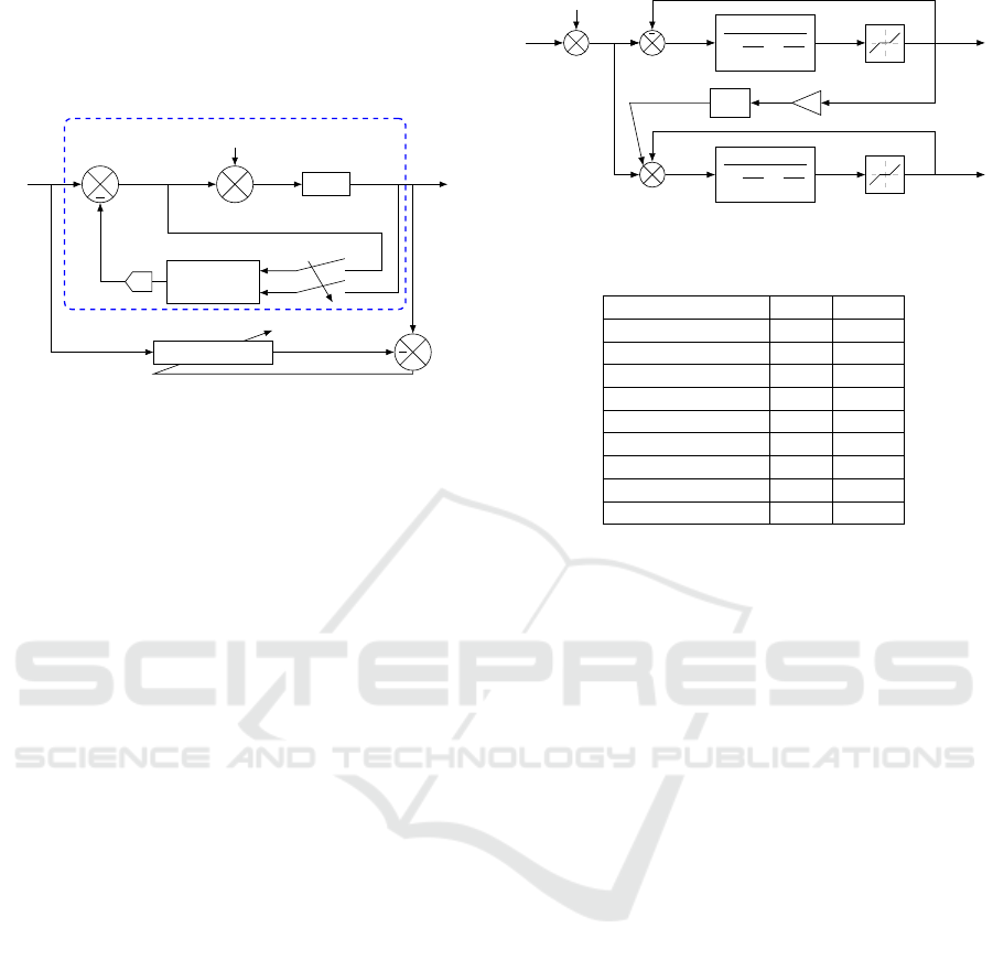
5 NUMERICAL EXAMPLE

In this section, the numerical example presented in

ﬁgure 9 (where s is the Laplace variable) is chosen to

illustrate the proposed approach. Table 1 gives all pa-

rameter values for this example. To show the generic-

ity of the model with regard to nonlinearities, the ex-

ample has been chosen to include differentiable and

non-differentiable nonlinearities. To begin with, the

inefﬁciency of the predictor trained without perturba-

tion in a disturbance environment is shown. More-

over, this predictor is not accurate when it is trained

with a disturbance if this disturbance varies or van-

ishes. Finally, the three steps deﬁned in ﬁgure 2 are

applied.

5.1 False Prediction in Case of

Disturbance

As said in the introduction section, the method pro-

posed in ﬁgure 1 leads to poor prediction results

when a disturbance appears and the predictor has

been trained using non-disturbed data. Figure 10(a)

2ξ

0,1

sin

2ξ

0,2

−

Figure 9: Studied system.

Table 1: Parameters.

Parameter Value Unit

2 -

0.5 -

0,1

150 rad.s

−1

4 -

0.05 -

0,2

300 rad.s

−1

−3

Start of the dead zones −0.2 -

End of the dead zones 0.2 -

presents prediction on undisturbed system (Γ = 0, in

ﬁgure 9) and ﬁgure 10(b) presents prediction on the

system disturbed by: Γ(t) = 0.2sin(2πt).

Figure 10(a) shows that the neural network is well

trained and gives accurate results in the nominal case

(Γ = 0). Figure 10(b) shows how the prediction is

affected by the input disturbance; ﬁrst output gives

acceptable results but second output prediction is far

from real data.

The next section will show that the same phe-

nomenon arises if the neural network is trained with a

disturbance.

5.2 Ofﬂine Training with a Disturbance

A neural network ofﬂine trained with a disturbance

cannot accurately predict the output if the disturbance

varies or vanishes. To this end, a FNN is trained on

the system presented in ﬁgure 9 with a sinusoidal in-

put disturbance ( f = 1Hz). Figure 11 presents the pre-

diction (obtained from the method explained in ﬁg-

ure 1) in the presence of the same disturbance, the

prediction without any disturbance and the prediction

with a sinusoidal input disturbance with f = 10Hz.

Figure 11 shows that the trained neural network

is speciﬁc to the sinusoidal input disturbance with

f = 1Hz as without any disturbance and for another

frequency the prediction is incorrect for the second

output and less accurate with regard to the ﬁrst input.

Section 5.1 and 5.2 have shown that using the

method presented in ﬁgure 1 leads to poor prediction

results in the face of varying disturbance proﬁles. The

Enhancing Neural Network Prediction against Unknown Disturbances with Neural Network Disturbance Observer

215

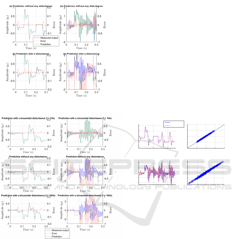
Figure 10: Inﬂuence of a disturbance on the prediction.

Figure 11: Inﬂuence of different disturbances on the predic-

tion.

following part corresponds to the proposed method to

enhance prediction against unknown disturbances.

5.3 Enhancing Prediction with the

Proposed Method

5.3.1 Ofﬂine Training of the State-Space Neural

Network

This section corresponds to the ﬁrst step of the

method described in ﬁgure 2. A SSNN with 50 neu-

rons in the hidden layer is chosen. The system has

been sampled at sampling time T

and we have used

10000 samples for the training set and 10000 samples

for the validation set. As explained previously, data

have been obtained without any disturbances, that is

Γ = 0 in ﬁgure 9, and have been normalized. The in-

put training sequence is constrained to [−1;1].

Figure 12 shows the results for training (several

runs have been performed but only the best result in

terms of cost function is presented) by presenting a

simulation on a test set which is different from the

training set. Regression, which corresponds to the

plot of the output of the model as a function of the

measured output, shows the training accuracy since it

is close to the ﬁrst bisector (for a perfect training the

regression would have been exactly on the ﬁrst bisec-

tor). It can be seen that the training is somewhat better

for the ﬁrst measure than it is for the second one. Us-

ing more neurons would lead to more accurate results.

0 0.2 0.4

Time (s)

-1

-0.5

0.5

Amplitude

Output 1

-2 -1 0 1 2

measured

-2

-1

Regression (Output 1)

-2 -1 0 1 2

measured

-2

-1

Regression (Output 2)

0 0.2 0.4

Time (s)

-2

-1

Amplitude

Output 2

Measure

SSNN Model

Figure 12: Learning results on a test scenario (different

from the training scenario).

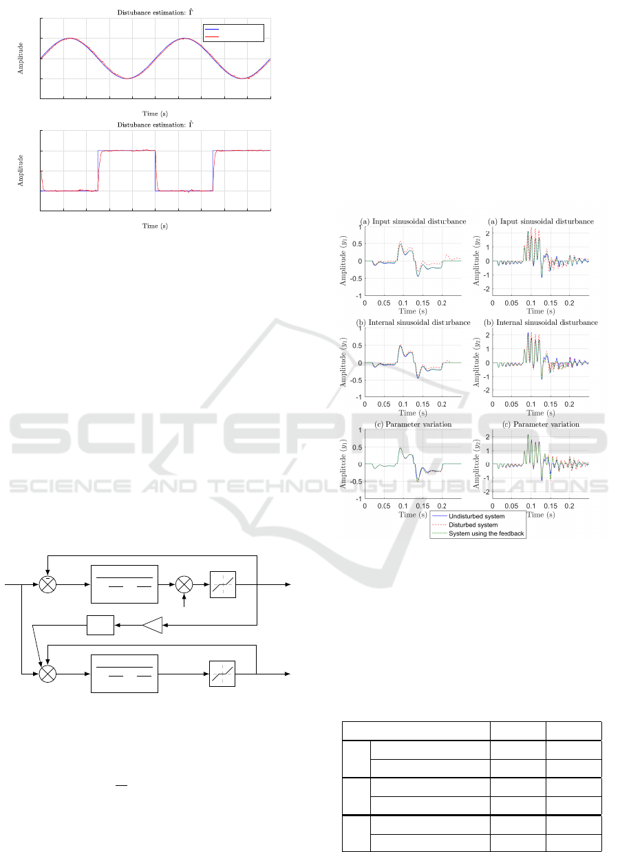
5.3.2 Extended Kalman Filter Implementation

The following part corresponds to the second step of

the method described in ﬁgure 2. We implement the

EKF by using a reasoning similar to the one done in

section 3.4 by using the SSNN model.

Experiment results done using the system pre-

sented in ﬁgure 9 are presented in ﬁgure 13 for two

different perturbations: the ﬁrst one corresponds to a

sinusoidal signal and the second one to a square sig-

nal.

The modelling error has a direct inﬂuence on

the estimated disturbance. The result shows that the

method is able to reconstruct the disturbance with a

good accuracy.

ICINCO 2019 - 16th International Conference on Informatics in Control, Automation and Robotics

216

0 0.2 0.4 0.6 0.8 1 1.2 1.4 1.6 1.8 2

-0.4

-0.2

0.2

0.4

0 0.2 0.4 0.6 0.8 1 1.2 1.4 1.6 1.8 2

-0.4

-0.2

0.2

0.4

Real disturbance

Estimation

Figure 13: Estimated disturbance.

5.3.3 Implementation of the Feedback

Compensator

The solution proposed in section 4 and ﬁgure 8 is now

tested to see the robustness of the plant against differ-

ent disturbances. It corresponds to the third step of

ﬁgure 2. Three kinds of experiments have been done:

the ﬁrst one corresponds to a system subject to an ad-

ditive sinusoidal disturbance input (Figure 6), the sec-

ond one to a system subject to an internal sinusoidal

disturbance for the ﬁrst measure (Figure 14) and the

last one corresponds to a parameter variation. Results

are respectively presented in ﬁgure 15 (a), (b) and (c).

For the case (c) the gain K

is multiplied by a factor

1.2 at time t = 0.125s in order to simulate an internal

parameter variation. Ideally, the solid blue line and

the dash-dot green line should be identical.

2ξ

0,1

sin

2ξ

0,2

−

Figure 14: Internal disturbance.

A cost function is introduced in order to compare

the invariance of the system as:

v,p

∑

i=1

I,p

− y

)

, (14)

where the index p refers the output p, y

I,p

is the out-

put of the disturbed system, corresponding to the dash

red line in ﬁgure 15 or the output of the system us-

ing the feedback, corresponding to the dash-dot green

line. Results are summed up in Table 2 where the

case (a),(b) and (c) correspond to those presented in

ﬁgure 15.

We can see from ﬁgure 15 (a-c) and Table 2 that

the system is less sensitive to disturbances even if the

disturbance applied to the plant is not an additive in-

put disturbance as considered in the model used in the

EKF. As shown with ﬁgure 13, the estimated distur-

bance also contains the model error thus, results pre-

sented in ﬁgure 15 can be improved if a better model

is used, which means using more neurons or by re-

training the neural network with other starting points.

Figure 15: Invariance of the system using the feedback

structure proposed in section 4.

Because the system is unvarying against distur-

bances, we can conclude that the global new system

can be modeled by a FNN trained online as it has been

done in (Bao et al., 2017). The predictor that arises

from this FNN will be less sensitive to disturbances

and thus be efﬁcient.

Table 2: Performance comparison.

Case I

v,1

v,2

(a)

Disturbed system 7.8 ∗ 10

−3

1.5 ∗ 10

−1

System using the feedback 1.0 ∗ 10

−4

1.1 ∗ 10

−2

(b)

Disturbed system 2.0 ∗ 10

−3

5.2 ∗ 10

−2

System using the feedback 3.7 ∗ 10

−4

2.8 ∗ 10

−2

(c)

Disturbed system 8.1 ∗ 10

−4

5.1 ∗ 10

−2

System using the feedback 6.3 ∗ 10

−4

4.4 ∗ 10

−2

Enhancing Neural Network Prediction against Unknown Disturbances with Neural Network Disturbance Observer

217

6 CONCLUSION

In this paper, a way to enhance neural network pre-

diction against unknown disturbances has been pre-

sented, thanks to a feedback structure that uses the

observed disturbance reconstructed by an extended

Kalman ﬁlter based on a state-space neural net-

work model. Numerical results obtained for a system

with non-differentiable and differentiable nonlineari-

ties have proven the interest in the proposed approach,

exhibiting satisfactory results in terms of prediction

errors and robustness against variations of the distur-

bance input proﬁles or parameter variations. These

results have been obtained at the price of a slight in-

crease in the predictor complexity, as the neural net-

work used for the prediction for the global system,

containing both the system and the observer, gener-

ally requires more neurons than a neural network pre-

dictor for the original system alone.

Future works will deal with improving learning

methods for SSNN and combining this work with the

Decoupled Extended Kalman Filter neural network

learning method (Puskorius and Feldkamp, 1997) in

order to get an adaptive ﬁlter. Other observer tech-

niques will also be tested in order to achieve a fair

comparison of the possible approaches. Finally, the

estimated disturbance can be used to obtain a distur-

bance predictor in the case of a control law design.

REFERENCES

Alessandri, A. (2000). Design of sliding-mode observers

and ﬁlters for nonlinear dynamic systems. In Proceed-

ings of the 39th IEEE Conference on Decision and

Control, volume 3, pages 2593–2598. IEEE.

Bao, X., Sun, Z., and Sharma, N. (2017). A recurrent neu-

ral network based MPC for a hybrid neuroprosthesis

system. In IEEE 56th Annual Conference on Decision

and Control, pages 4715–4720. IEEE.

Bullinger, E. and Allg

ower, F. (1997). An adaptive high-

gain observer for nonlinear systems. In 36th IEEE

Conference on Decision and Control, pages 4348–

4353.

Chen, W.-H., Ballance, D. J., Gawthrop, P. J., and O’Reilly,

J. (2000). A nonlinear disturbance observer for robotic

manipulators. IEEE Transactions on industrial Elec-

tronics, 47(4):932–938.

Cybenko, G. (1989). Approximation by superpositions of

a sigmoidal function. Mathematics of control, signals

and systems, 2(4):303–314.

De Jesus, O. and Hagan, M. T. (2007). Backpropagation al-

gorithms for a broad class of dynamic networks. IEEE

Transactions on Neural Networks, 18(1):14–27.

Diaconescu, E. (2008). The use of narx neural networks

to predict chaotic time series. Wseas Transactions on

computer research, 3(3):182–191.

Gavin, H. (2017). The levenberg-marquardt method for

nonlinear least squares curve-ﬁtting problems. De-

partment of Civil and Environmental Engineering,

Duke University.

Grossman, W. D. (1999). Observers for discrete-time non-

linear systems.

Hagan, M. T., Demuth, H. B., Beale, M. H., et al. (1996).

Neural network design, volume 20. Pws Pub. Boston.

Haykin, S. (2004). Kalman ﬁltering and neural networks,

volume 47. John Wiley & Sons.

Hedjar, R. (2013). Adaptive neural network model predic-

tive control. International Journal of Innovative Com-

puting, Information and Control, 9(3):1245–1257.

Kalman, R. E. (1960). A new approach to linear ﬁltering

and prediction problems. Journal of basic Engineer-

ing, 82(1):35–45.

Keviczky, T. and Balas, G. J. (2006). Receding horizon con-

trol of an f-16 aircraft: A comparative study. Control

Engineering Practice, 14(9):1023–1033.

Lakhal, A., Tlili, A., and Braiek, N. B. (2010). Neural net-

work observer for nonlinear systems application to in-

duction motors. International Journal of Control and

Automation, 3(1):1–16.

Levenberg, K. (1944). A method for the solution of cer-

tain non-linear problems in least squares. Quarterly

of applied mathematics, 2(2):164–168.

Marquardt, D. W. (1963). An algorithm for least-squares

estimation of nonlinear parameters. Journal of

the society for Industrial and Applied Mathematics,

11(2):431–441.

Pascanu, R., Mikolov, T., and Bengio, Y. (2013). On the

difﬁculty of training recurrent neural networks. In In-

ternational Conference on Machine Learning, pages

1310–1318.

Puskorius, G. and Feldkamp, L. (1997). Extensions and en-

hancements of decoupled extended kalman ﬁlter train-

ing. In International Conference on Neural Networks,

volume 3, pages 1879–1883. IEEE.

Talebi, H. A., Abdollahi, F., Patel, R. V., and Khorasani,

K. (2010). Neural network-based state estimation

schemes. In Neural Network-Based State Estimation

of Nonlinear Systems, pages 15–35. Springer.

Terejanu, G. A. (2008). Extended kalman ﬁlter tutorial. De-

partment of Computer Science and Engineering, Uni-

versity at Buffalo.

Vatankhah, B. and Farrokhi, M. (2017). Nonlinear model-

predictive control with disturbance rejection prop-

erty using adaptive neural networks. Journal of the

Franklin Institute, 354(13):5201–5220.

Wan, E. A. and Van Der Merwe, R. (2000). The unscented

kalman ﬁlter for nonlinear estimation. In Adaptive

Systems for Signal Processing, Communications, and

Control Symposium, pages 153–158. IEEE.

Werbos, P. (1974). Beyond regression: New tools for pre-

diction and analysis in the behavioral sciences. Ph. D.

dissertation, Harvard University.

Werbos, P. J. (1990). Backpropagation through time: what

it does and how to do it. Proceedings of the IEEE,

78(10):1550–1560.

ICINCO 2019 - 16th International Conference on Informatics in Control, Automation and Robotics

218

Williams, R. J. and Zipser, D. (1989). A learning algo-

rithm for continually running fully recurrent neural

networks. Neural computation, 1(2):270–280.

Yu, D. and Gomm, J. (2003). Implementation of neural

network predictive control to a multivariable chemical

reactor. Control Engineering Practice, 11(11):1315–

1323.

Zamarre

no, J. M. and Vega, P. (1998). State space neural

network. properties and application. Neural networks,

11(6):1099–1112.

Enhancing Neural Network Prediction against Unknown Disturbances with Neural Network Disturbance Observer

219