A PGD-based Method for Robot Global Path Planning: A Primer
N. Mont
´
es
1 a
, F. Chinesta
2
, A. Falc
´
o
1 b
, M. C. Mora
3 c
, L. Hilario
1 d
and J. L. Duval
4
1
Department of Physics, Mathematics and Technological Sciences, University CEU Cardenal Herrera,
46115, Alfara del Patriarca, Spain
2
PIMM, ENSAM ParisTech ESI GROUP Chair on Advanced Modeling and Simulation of Manufacturing Processes,
Paris, France
3
Department of Mechanical Engineering and Construction, Universitat Jaume I, Castell
´
on, Spain
4
ESI Group, RUNGIS CEDEX, France
Keywords:
Model Order Reduction Techniques, PGD, Path Planning, Potential Field Methods, Laplace Equation.
Abstract:
The present paper shows, for the first time, the technique known as PGD-Vademecum as a global path planner
for mobile robots. The main idea of this method is to obtain a Vademecum containing all the possible paths
from any start and goal positions derived from a harmonic potential field in a predefined map. The PGD is a
numerical technique with three main advantages. The first one is the ability to bring together all the possible
Poisson equation solutions for all start and goal combinations in a map, guaranteeing that the resulting potential
field does not have deadlocks. The second one is that the PGD-Vademecum is expressed as a sum of uncoupled
multiplied terms: the geometric map and the start and goal configurations. Therefore, the harmonic potential
field for any start and goal positions can be reconstructed extremely fast, in a nearly negligible computational
time, allowing real-time path planning. The third one is that only a few uncoupled parameters are required
to reconstruct the potential field with a low discretization error. Simulation results are shown to validate the
abilities of this technique.
1 INTRODUCTION
An essential in robotics is to guide the robot safely
from a start to a goal position among a set of ob-
stacles. For this purpose, a collision-free path must
be generated, which implies a computationally hard
geometric path planning unfeasible in real-time (RT)
applications (Reif, 1979). This problem is known
in the literature as motion planning or the piano
mover’s problem and its complexity has motivated
a lot of research works in the field of robot path
planning. Some works have studied subproblems of
the general approach (Kavraki and LaValle, 2008).
Other researchers have considered alternative plan-
ning paradigms under simplified but realistic assump-
tions such as, for instance, sampling-based planners,
grid-based searches, interval-based searches, geomet-
ric algorithms, etc (Kavraki and LaValle, 2008).
a
https://orcid.org/0000-0002-0661-3479
b
https://orcid.org/0000-0001-6225-0935
c
https://orcid.org/0000-0003-0627-6764
d
https://orcid.org/0000-0003-0729-6628
One of the most used algorithm is the Artificial
Potential Field method (APF), (Khatib, 1986). This
technique defines an artificial potential field in the
configuration space (C-space) that generates a path
from a start to a goal position. This method is very
fast for RT applications. However, the robot could get
stuck in a local minimum of the potential function.
This problem can be solved using harmonic functions
in the generation of the potential field (Canny, 1998),
which satisfy the Laplace equation in the C-space
and completely eliminate local minima as they sat-
isfy the Min-Max principle (Rimon and Koditschek,
1992). These functions were initially proposed in
(Zhachmanoglou and Thoe, 1986) and used for robot
path planning in (Connolly et al., 1990; Kim and
Khosla, 1992; Akishita et al., 1993; Guldner et al.,
1997; Waydo and Murray, 2003; Rosell and Iniguez,
2002; Saudi and Sulaiman, 2012). The main prob-
lem of this technique, addressed in (Waydo and Mur-
ray, 2003), is that the solution must be numerically
computed in a discrete mesh and, therefore, the com-
putational cost increases exponentially with the mesh
resolution. In (Gingras et al., 2010), one of the last
Montés, N., Chinesta, F., Falcó, A., Mora, M., Hilario, L. and Duval, J.
A PGD-based Method for Robot Global Path Planning: A Primer.
DOI: 10.5220/0007809000310039
In Proceedings of the 16th International Conference on Informatics in Control, Automation and Robotics (ICINCO 2019), pages 31-39
ISBN: 978-989-758-380-3
Copyright
c
 2019 by SCITEPRESS – Science and Technology Publications, Lda. All rights reserved
31

studies, an scanned environment composed by 1500
triangles had a computational cost of 19.2 Sec in a
laptop Dell latitude with an Intel Core 2 Processor,
2GB RAM, inadmissible for RT applications.
More recently, in the field of advanced computa-
tional methods, a novel alternative called Proper Gen-
eralized Decomposition (PGD) has appeared to com-
pute the Laplace equation. It is a completely new ap-
proach for solving classic high-complexity problems
(Chinesta et al., 2013; Chinesta et al., 2014). Many
difficult problems can be efficiently converted into a
multidimensional framework, which opens up novel
possibilities to solve old and new problems with ap-
proaches not foreseen until now. In a PGD frame-
work, the model can be solved only once with the aim
of obtaining a general solution that includes all the
solutions for every value of the parameters, that is, a
Computational Vademecum.
The goal of the present paper is to present the
computation of a PGD-based computational Vademe-
cum (PGD-Vademecum for short) for using the poten-
tial flow theory based on harmonic functions in two
RT path planning applications. This paper is orga-
nized as follows. Section 2 introduces the potential
flow theory and obtains a harmonic function derived
from the Laplace equation. In Section 3, a specific
PGD-Vademecum for robot path planning is calcu-
lated and a numerical example is used to demonstrate
the benefits of the method. In Section 4, some sim-
ulation examples are provided. Finally, in Section 5
conclusions and future works are presented.
2 BACKGROUND
2.1 Path Planning based on the
Potential Flow Theory
During the last years, many path planning tecnhiques
have been based on the potential flow theory (Con-
nolly et al., 1990; Kim and Khosla, 1992; Akishita
et al., 1993; Guldner et al., 1997; Waydo and Mur-
ray, 2003; Rosell and Iniguez, 2002; Saudi and Su-
laiman, 2012; Gingras et al., 2010), focused mainly
in the resolution of the Laplace equation. First of all,
let us outline the mathematical model describing the
flow of an inviscid incompressible fluid. Assuming
a steady state irrotational flow in the Eulerian frame-
work, the velocity υ obeys the relation
5 × υ = 0, (1)
and hence the velocity is the gradient of a scalar po-
tential function, i.e. υ = ∇u. Then the potential u ap-
pears as a solution of the Laplace equation:
∆ u = 0. (2)
By using a 2.5D mould filling model similar to
(Dom
´
enech et al., 2016) it is possible to introduce a
localized fluid source (respectively, sink) modelled by
a Dirac term δ
S
(respectively, −δ
T
) added to the right
hand side of (2). To this end we assume a unit amount
of fluid injected at point S during a unit of time and
the same unit withdrawn at point T, the velocity of the
fluid is now the solution of the Poisson equation, that
includes the source term f = δ
S
− δ
T
as:
−∆u = δ
S
− δ
T
. (3)
Equation (3) must be complemented by appropriate
boundary conditions. In these sense, the fluid cannot
flow through the boundaries, a condition expressed by
υ · n (n being a vector normal to the boundary Γ). On
Γ the velocity must verify:
−∇u · n = 0, (4)
which is the usual the Neumann boundary condition
expressed by
∂u
∂n




Γ
= 0. (5)
The resolution of the Poisson equation under these
conditions produces a potential field from the Starting
point S (source) to the Target point T (sink), without
deadlocks (Gingras et al., 2010).
2.2 Resolution of the Poisson Equation
using PGD
Consider the two dimensional Poisson equation
∆u(x, y) = f (x, y) (6)
over a two-dimensional rectangular domain Ω
X
=
Ω
X
× Ω
Y
⊂ R
2
with boundary condition
∂u
∂n



Γ
= q.
For all suitable test functions u
∗
, the weighted resid-
ual forms reads
Z
Ω
X
u
∗
· (∆u − f )dΩ
X
(7)
The classical way of accounting for Neuman con-
ditions is to integrate by parts the weighted residual
form and implement the flux condition as a so-called
natural boundary condition:
Z
Ω
X
∇u
∗
· ∇udΩ
X
=
Z
Ω
X
u
∗
· f dΩ
X
−
Z
Ω
X
u
∗
(x, y = Γ) · q dΩ
X
(8)
ICINCO 2019 - 16th International Conference on Informatics in Control, Automation and Robotics
32

Our goal is to obtain a PGD approximate solution to
(8) in the separated form
u(Ω
X
) =
N
∑
i=1
X
i
(x) ·Y
i
(y) (9)
We shall do so by computing each term of the expan-
sion one at a time, thus enriching the PGD approxima-
tion until a suitable convergence criterion is satisfied.
At each enrichment step n, (n > 1), we have already
computed the n−1 first terms of the PGD approxima-
tion (9):
u
n−1
(Ω
X
) =
n−1
∑
i=1
X
i
(x) ·Y
i
(y) (10)
We now wish to compute the next term X
n
(x) · Y
n
(y)
to obtain the enriched PGD solution
u
n
(x, y) = u
n−1
(x, y) + X
n
(x) ·Y
n
(y) =
=
n−1
∑
i=1
X
i
(x) ·Y
i
(y) + X
n
(x) ·Y
n
(y)
(11)
Both functions X
n
(x) and Y
n
(y) are unknown at the
current enrichment step n and an alternative iterative
scheme is applied. We use index p to denote a partic-
ular iteration.
u
n, p
(x, y) = u
n−1
(x, y) + X
p
n
(x) ·Y
p
n
(y) (12)
The simplest one is an alternating direction strategy
that computes X
p
n
(x) from Y
p−1
n
(y) and then Y
p
n
(y)
from X
p
n
(x). An arbitrary initial guess Y
0
n
(y) is spec-
ified to start the iterative process. The non-linear it-
erations proceed until reaching a fixed point within
a user-specified tolerance, see (Chinesta et al., 2013;
Chinesta et al., 2014). The convergence of the above
procedure to the weak solution of (6) is proved in
(Falc
´
o and Nouy., 2012).
3 PATH PLANNING BASED ON
THE PGD-VADEMECUM
The preceding section has presented a simple example
application of the resolution of the Poisson equation
using PGD in a case where the 2D space is decom-
posed in X and Y . (Chinesta et al., 2013; Chinesta
et al., 2014) demonstrate that parameters in a model
can be set as additional coordinates when using the
PGD approach. In the following sections, a path plan-
ning example is presented where these additional co-
ordinates are all the possible combinations of the start
and target positions and can be included in the source
term of the Poisson equation (6) .
3.1 Definition of the Source Term
First of all, it is necessary to assume that a con-
stant source term f in equation (6) is actually a non-
uniform source term f (Ω
X
, Ω
S
, Ω
T
), where Ω
X
=
Ω
x
× Ω
y
, Ω
S
= Ω
r
× Ω
s
and Ω
T
= Ω
r
× Ω
t
. In this
definition, the start and target points S and T are de-
fined by means of Gaussian models with mean and
variance: S = (s, r) and T = (t, r), respectively. In
these models, s and t are the mean values located
in specific points X = (x, y) in each separated space
Ω
S
, Ω
T
and r is the variance. Gaussian models are
used instead of Delta Dirac models because they pro-
vide much better results in a PGD-Vademecum than
Delta Dirac model, as explained in (Chinesta et al.,
2013). In order to define the source term, the next
two matrices must be constructed first:
f (X, S) =



f (x
1
, s
1
) . . . f (x
1
, s
N
)
.
.
.
.
.
.
.
.
.
f (x
N
, s
1
) . . . f (x
N
, s
N
)



f (X, T ) =



f (x
1
, t
1
) . . . f (x
1
, t
N
)
.
.
.
.
.
.
.
.
.
f (x
N
, t
1
) . . . f (x
N
, t
N
)



(13)
Applying the Single Value Decomposition (SVD)
method to these matrices, the result is the decomposi-
tion of the source term in the form:
f (X, S) =
F
∑
j=1
α
S
j
· F
S
j
(X) · G
S
j
(S)
g(X, T ) =
F
∑
j=1
α
T
j
· F
T
j
(X) · G
T
j
(T )
(14)
Thus, the Poisson equation to be solved results in the
form:
∆u(x, y) = f (X, S) + g(X, T ) (15)
3.2 Computation of the
PGD-Vademecum
For all suitable test functions u
∗
, the weighted resid-
ual forms reads
Z
Ω
X,S,T
u
∗
· (∆u − f )dΩ
X,S,T
= 0 (16)
where f is in the form obtained in (15):
f = f (X, S) + g(X, T ) (17)
A PGD-based Method for Robot Global Path Planning: A Primer
33

Now, equation (8) reads
Z
Ω
X,S,T
5u
∗
· 5udΩ
X,S,T
=
Z
Ω
X,S,T
u
∗
· f dΩ
X,S,T
−
−
Z
Ω
X
,S,T
u
∗
(x, y = Γ) · q dΩ
X,S,T
(18)
and the PGD-Vademecum is now
u(X, S, T ) =
N
∑
i=1
R
i
(X) · W
i
(S) · K
i
(T ) (19)
From now on, it will be assumed that the common
variance r takes a fixed value and the construction of
the Vademecum will be obtained considering the so-
lution of (15) for that value r and all the values of
(X = (x, y); S = (s
1
, s
2
);T = (t
1
, t
2
)) ∈ Ω
X
× Ω
S
× Ω
T
.
Then, the PGD-Vademecum solution is con-
structed considering that
u
n−1
(X, S, T ) =
n−1
∑
i=1
R
i
(X) · W
i
(S) · K
i
(T ) (20)
where the enrichment step is given by
u
n
= u
n−1
+ R(X) · W (S) · K(T ). (21)
The key point is to find a rank-one function in the
form
R(X) · W (S) · K(T ) =
R
1
(x) · R
2
(y) ·W
1
(s
1
) ·W
2
(s
2
) · K
1
(t
1
) · K
2
(t
2
)
(22)
which satisfies
Z
Ω
X
×Ω
S
×Ω
T
u
∗
· (∆u
n
− f ) dΩ
X,S,T
= 0
for all u
∗
in the linear space of functions
R(X) · W (S) · K
∗
(T ) + R(X) · W
∗
(S) · K(T )
+R
∗
(X) · W (S) · K(T ),
where K
∗
(T ) is orthogonal to K(T ),W
∗
(S) is or-
thogonal to W (S) and R
∗
(X) is orthogonal to R(X ).
In the appendix an alternating direction algorithm is
provided to construct the separated representation. A
prior step implies the discretization of (20) by means
of the Finite-Element Method (FEM) with
N
x
· N
y
+ N
s
1
· N
s
2
+ N
t
1
· N
t
2
degrees of freedom and assuming that
N = N
x
= N
y
= N
s
1
= N
s
2
= N
t
1
= N
t
2
.
Therefore, at each iteration step, the algorithm com-
putes the 3N
2
terms of the rank-one update (22) and,
after n iterations, the PGD approximation of the solu-
tion u is given by (21).
3.3 A Simple Numerical Example
With the aim of testing the advantages of the PGD
framework, a simple example is developed in this sub-
section. Let us consider a domain Ω
X
of 5m × 5m
square. Let us select a discretization of the domain
using N
x
= N
y
= 50 nodes on each side, that is, 2500
degrees of freedom and the variance r set to 1.2. In
Figure 1 an example for S = (1, 4) and T = (4, 1) is
shown. The left column displays the source term and
the right column shows the resulting PGD reconstruc-
tion for n = 200 terms.
The computational cost of the PGD reconstruction
is 0.0101s in a Mac with an Intel Core 2 Duo Proces-
sor (3.06 GHz) and 4 GB RAM. It is worth noting
the difference between this negligible value and the
cost of a FEM approximation to solve a standard lin-
ear system, where the computational cost increases to
4.7s.
3.4 Residual Error of the PGD
Approximation
The error of the PGD approximation versus the num-
ber of terms used can be measured by means of dif-
ferent techniques. A very appropriate error estimator
in this case is the L
2
(Ω
X
× Ω
S
× Ω
T
)-residual R(n),
that can be obtained inserting the PGD-Vademecum
approximation in the Poisson equation, resulting in
R(n) =
Z
Ω
X
×Ω
S
×Ω
T
(∆u
n
− f ) · (∆u
n
− f ) dΩ
X,S,T
(23)
Figure 2 shows one of the most important features
of the PGD: the relevant information is stored in the
first terms of the approximation.
3.5 Local Minima in the Approximated
Solution
The use of harmonic functions solve the problem of
local minima still present in APF-based techniques.
The solution of an harmonic function based on flow
dynamics and described by the Poisson equation is
approximated in the present paper by means of the
PGD-Vademecum technique. Therefore, this approx-
imation could produce local minima in the solution
if the variance value r is not adjusted properly. For
the numerical example developed in the previous sub-
sections, Figure 4 shows the maximum number of lo-
cal minima of the PDG solution for all the possible
Start and Target combinations (50
4
) and for different
variance values (r =0.1, 0.3, 0.5 and 0.7). A spe-
cific node (N
1
, N
2
) is defined as a local minima if the
ICINCO 2019 - 16th International Conference on Informatics in Control, Automation and Robotics
34

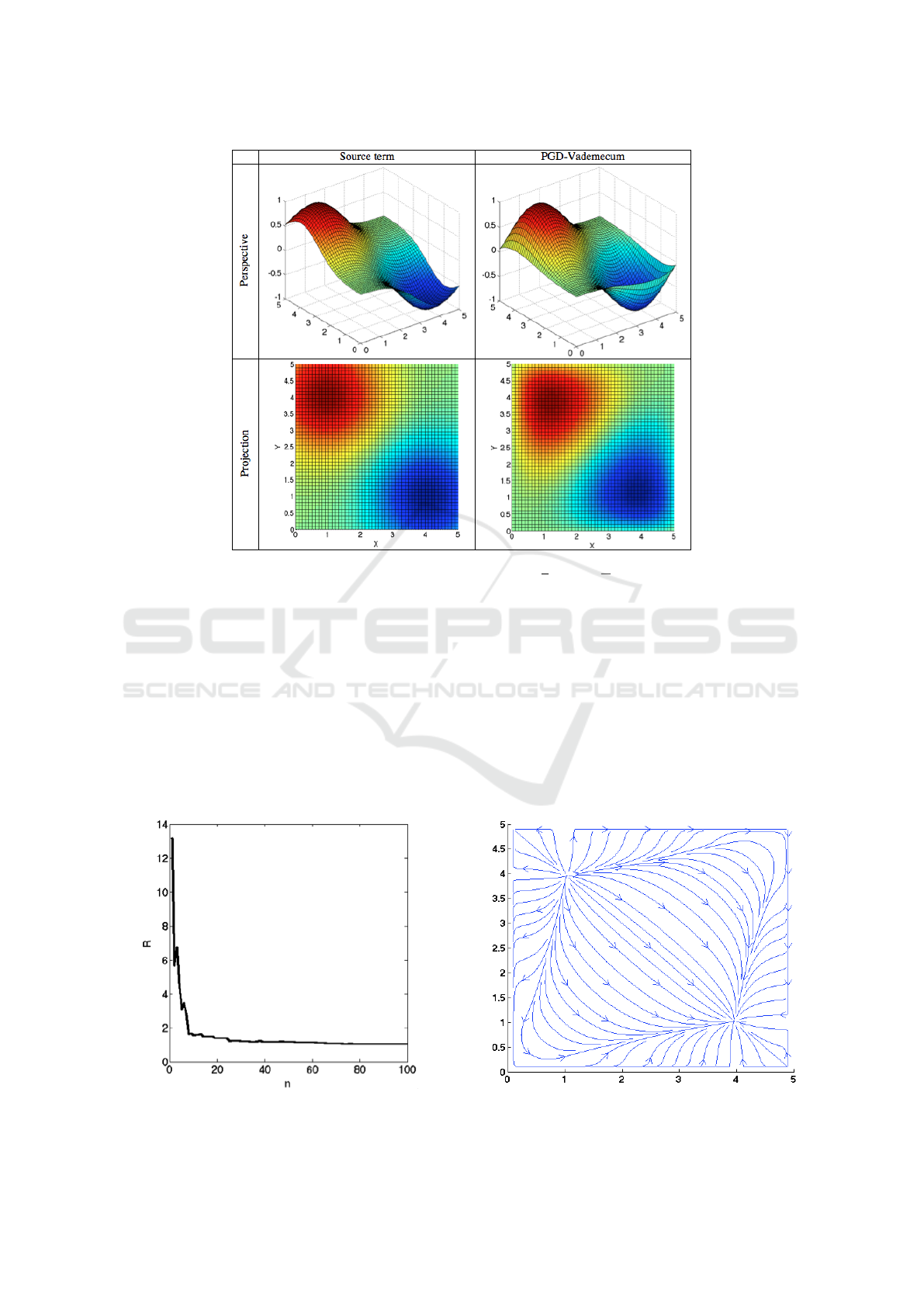
Figure 1: PGD reconstruction VS source term for S = (1, 4), T = (4, 1).
eight surrounding nodes have an u value greater than
its u value. As displayed in Figure 4, a free-of-local-
minima PGD-Vademecum approximation can be ob-
tained if the selected variance value is higher that 0.7.
3.6 Computation of Streamlines
As explained in Section 1, the use of harmonic func-
tions solve the problem of local minima present in
APF-based techniques. Harmonic functions are based
on flow dynamics, described by the Poisson equation,
Figure 2: Residual error versus number of PGD terms.
where the potential field is free of local minima and
derives in a set of streamlines (Connolly et al., 1990;
Kim and Khosla, 1992; Akishita et al., 1993; Guld-
ner et al., 1997; Waydo and Murray, 2003; Rosell and
Iniguez, 2002; Saudi and Sulaiman, 2012; Gingras
et al., 2010). These flow lines are independent of time
and describe the direction of a massless fluid element
that travels from an initial to a final position, follow-
ing a velocity field that can be obtained from the gra-
dient of the potential field, as described in equations
(25).
Figure 3: Streamlines.
A PGD-based Method for Robot Global Path Planning: A Primer
35

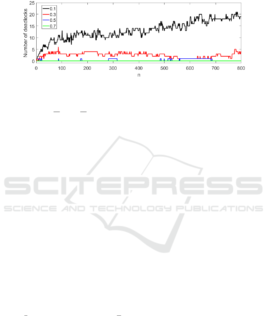
Figure 4: Local minima in the PGD approximation solution.
v
x
=
du
dx
, v
y
= −
du
dy
(24)
Then, from the velocity field, any interpolation
technique can be used to compute the streamlines as,
for instance, linear, cubic, splines, etc. Fig 3 displays
the streamlines that result from using linear interpo-
lation for the PGD reconstruction showed in Figure
1.
4 REAL-TIME APPLICATION
(SHORTEST PATH)
Some RT simulations in Matlab have been performed
with the aim of testing the advantages that the PGD-
Vademecum approach offers. An omnidirectional
mobile robot has been modelled that navigates in a
5x5m square environment guided by a harmonic po-
tential field approximated by the PGD with 50× 50
nodes, r = 0.7 and n = 200. For a realistic imple-
mentation, only as small Region Of Interest (ROI) is
reconstructed in each algorithm execution. The ROI
is composed of the surrounding nodes of the current
robot position and its size depends on the maximum
robot velocity. In the present example, for particu-
lar Start and Target configurations, the robot selects
the shortest streamline, which is a straight line head-
ing to the Target. Figure 5 depicts different trajec-
tories followed by the robot beginning at the start-
ing point S = (1, 4) to subsequent target points T =
(4, 1), (3, 4), (2, 1), (4, 3).
A second example is also presented in the same
5x5m square environment, potential function and pa-
rameters. This time, an static obstacle in located in the
environment. For a specific Start and Target configu-
ration, it can be seen that the robot selects the shortest
streamline heading to the Target and avoiding the ob-
stacle. Figure 6 depicts the simulation results.
5 CONCLUSIONS AND FUTURE
WORKS
The present paper develops, for the first time, the ap-
plication of the numerical technique known as PGD-
Vademecum in the global path planning problem for
mobile robotics. This method generates a sort of
Computational Vademecum containing all the possi-
ble robot paths for any Start and Target combinations
in a predefined map. This PGD-Vademecum must be
computed off-line and stored in the robot memory in
order to be reconstructed on-line for any particular
combination of start and target configurations. It is
very fast for RT applications because its formulation
results in a simple sum of products. In addition, dur-
ing navigation tasks, only the surrounding nodes of
the robot position need to be reconstructed in every
algorithm execution. As a result, the computational
costs in RT are extremely low, almost negligible. The
robot paths obtained are based on the Laplace/Poisson
equation and, thus, are local-minima free when the
variance is properly adjusted in the PGD approxi-
mated solution. This property makes the proposed ap-
proach a promising method to solve the piano mover’s
problem. The only drawback noticed is the generation
of a small offset in the start and target positions due
to the definition of the source term, as start and target
positions have a coupling effect. The solution of this
problem is our immediate future work.
REFERENCES
Akishita, S., Hisanobu, T., and Kawamura, S. (1993). Fast
path planning available for moving obstacle avoidance
by use of laplace potential. IEEE/RSJ Int. Conf. on
Intelligent Robots and Systems, 1(1):673–678.
Canny, J. (1998). The complexity of robot motion planning.
MIT press, Cambridge, Massatchusetts.
Chinesta, F., Keunings, R., and Leygue, A. (2014). The
ICINCO 2019 - 16th International Conference on Informatics in Control, Automation and Robotics
36

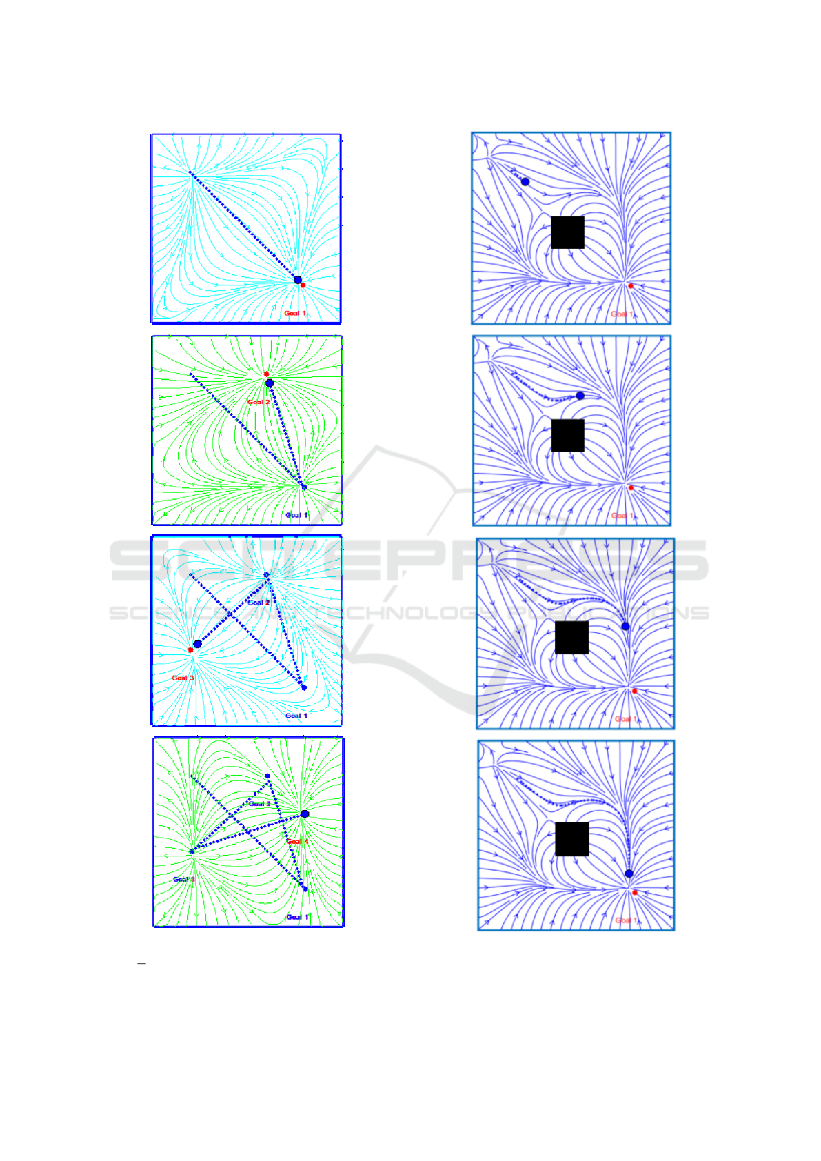
Figure 5: Simulation results: the robot visits the following
targets T = (4, 1), (3, 4), (2, 1), (4, 3).
Figure 6: Simulation results: the robot navigates to the tar-
get avoiding an obstacle in the environment.
A PGD-based Method for Robot Global Path Planning: A Primer
37

Proper Generalized Decomposition for Advanced Nu-
merical Simulations. Springer Briefs in Applied Sci-
ence and Technology, Berlin, 2nd edition.
Chinesta, F., Leygue, A., Bordeu, F., Aguado, J., Cueto,
E., Gonzalez, D., Alfaro, I., Ammar, A., and Huerta,
A. (2013). Pgd-based computational vademecum for
efficient design, optimization and control. Archives of
Computational Methods in Engineering, 20(1):31–59.
Connolly, C., Burns, J., and Weiss, R. (1990). Path planning
using laplace’s equation. IEEE Int. Conf. on Robotics
and Automation, 1(1):2102–2106.
Dom
´
enech, L., Falc
´
o, A., Garc
´
ıa, V., and S
´
anchez, F.
(2016). Towards a 2.5d geometric model in mold fill-
ing simulation. Journal of Computational and Applied
Mathematics, 29(1):183–196.
Falc
´
o, A. and Nouy., A. (2012). Proper generalized decom-
position for nonlinear convex problems in tensor ba-
nach spaces. Numerische Mathematik, 121(3):503–
530.
Gingras, D., Dupuis, E., Payre, G., and Lafontaine., J.
(2010). Path planning based on fluid mechanics for
mobile robots used unstructured terrain models. IEEE
International Conference on Robotics and Automa-
tion, 1(1):1978–1984.
Guldner, J., Utkin, V. I., and Hashimoto, H. (1997). Robot
obstacle avoidance in n-dimensional space using pla-
nar harmonic artificial fields. Journal of Dynamic Sys-
tems, Measurement and Control, 119(2):119–160.
Kavraki, L. and LaValle, S. (2008). Chapter 5. Motion
Planning, Handbook of Robotics. Siciliano, Khatib
(Eds), Springer, Berlin, 2nd edition.
Khatib, O. (1986). Real-time obstacle avoidance for ma-
nipulators and mobile robots. International Journal
of Robotic Research, 1(1):90–98.
Kim, J. and Khosla, P. (1992). Real-time obstacle avoidance
using harmonic potencial functions. IEEE Transac-
tions on Robotics and Automation, 8(3):338–349.
Reif, J. (1979). Complexity of the mover’s problem and
generalizations. IEEE Symp. Found. Comput. Sci.,
pages 421–427.
Rimon, E. and Koditschek, D. (1992). Exact robot naviga-
tion using artificial potential functions. IEEE Trans-
actions on Robotics and Automation, 8(5):501–518.
Rosell, J. and Iniguez, P. (2002). A hierarchical and dy-
namic method to compute harmonic functions for con-
strained motion planning. IEEE/RSJ Int. Conf. on In-
telligent Robots and Systems, 1(1):2335–2340.
Saudi, A. and Sulaiman, J. (2012). Path planing for
mobile robots using 4egsor via nine-point laplacian
(4egsor9l) iterative method. International Journal of
computer applications., 53(16):38–42.
Waydo, S. and Murray, S. (2003). Vehicle motion planning
using stream functions. IEEE Int. Conf. on Robotics
and Automation, 1(1):2484–2491.
Zhachmanoglou, E. and Thoe, D. (1986). Introduction to
partial differential equations with applications. Balti-
more Williams & Wilkins, Baltimore.
APPENDIX: Alternating Directions
Separated Representation
Constructor
Computing R(X
) from W (S), K(T )
Z
Ω
X,S,T
dR
∗
dR
∗
dR
dR
W
2
K
2
+ R
∗
R

dW
dW

2
K
2
+ R
∗
RW
2
·
·

dK
dK

2
dΩ
X,S,T
= −
Z
Ω
X,S,T
n−1
∑
i=1
dR
∗
dR
∗
dR
i
dR
i
W W
i
K K
i
+
+ R
∗
R
i
dW
dW
dW
i
dW
i
K K
i
+ R
∗
R
i
W W
i
dK
dK
dK
i
dK
i
dΩ
X,S,T
−
−
Z
Ω
X,S,T
R
∗
W K ( f (X, S) + g(X , T )) dΩ
X,S,T
−
−
Z
Ω
X,S,T
R
∗
(Γ)W K q dΩ
X,S,T
(25)
Taking into account the following notation for the
known terms
w
1
=
Z
Ω
S
W
2
d
Ω
S
w
5
=
Z
Ω
S
W G
S
j
d
Ω
S
t
3
=
Z
Ω
T
K K
i
d
Ω
S
w
2
=
Z
Ω
S

dW
dW

2
d
Ω
S
w
6
=
Z
Ω
S
W d
Ω
S
t
4
=
Z
Ω
T
dK
dK
dK
i
dK
i
d
Ω
T
w
3
=
Z
Ω
S
W W
i
d
Ω
S
t
1
=
Z
Ω
T
K
2
d
Ω
S
t
5
=
Z
Ω
T
K G
T
j
d
Ω
T
w
4
=
Z
Ω
S
dW
dW
dW
i
dW
i
d
Ω
S
t
2
=
Z
Ω
T

dK
dK

2
d
Ω
T
t
6
=
Z
Ω
T
K d
Ω
T
(26)
Equation 25 is reduced to
Z
Ω
X
dR
∗
dR
∗
dR
dR
w
1
t
1
+ R
∗
Rw
2
t
1
+ R
∗
Rw
1
t
2
dΩ
X
=
−
Z
Ω
X
n−1
∑
i=1
dR
∗
dR
∗
dR
i
dR
i
w
3
t
3
+ R
∗
R
i
w
4
t
3
+ R
∗
R
i
w
3
t
4
dΩ
X
+
+
Z
Ω
X
R
∗
F
∑
j=1
w
5
t
6
α
S
F
S
(X) +t
5
w
6
α
T
F
T
(X)
!
dΩ
X
−
− w
6
t
6
q
Z
Ω
X
R
∗
(Γ)dΩ
X
(27)
ICINCO 2019 - 16th International Conference on Informatics in Control, Automation and Robotics
38

Computing W (S) from R(X), K(T )
Z
Ω
X,S,T

dR
dR

2
W
∗
W K
2
+ R
2
dW
∗
dW
∗
dW
dW
K
2
+ R
2
W
∗
W ·
·

dK
dK

2
dΩ
X,S,T
= −
Z
Ω
X,S,T
n−1
∑
i=1
dR
dR
dR
i
dR
i
W
∗
W K K
i
+
+ RR
i
dW
∗
dW
∗
dW
i
dW
i
K K
i
+ RR
i
W
∗
W
i
dK
dK
dK
i
dK
i
dΩ
X,S,T
−
−
Z
Ω
X,S,T
RW
∗
K ( f (X, S) + g(X, T ))dΩ
X,S,T
−
−
Z
Ω
X,S,T
R(Γ)W
∗
K q dΩ
X,S,T
(28)
Taking into account the following notation for the
known terms
r
1
=
Z
Ω
X
R
2
d
Ω
X
r
6
=
Z
Ω
X
RF
T
j
d
Ω
X
t
4
=
Z
Ω
T
dK
dK
dK
i
dK
i
d
Ω
T
r
2
=
Z
Ω
X

dR
dR

2
d
Ω
X
r
7
=
Z
Ω
X
R(Γ)d
Ω
X
t
5
=
Z
Ω
T
K G
T
j
d
Ω
T
r
3
=
Z
Ω
X
RR
i
d
Ω
X
t
1
=
Z
Ω
T
K
2
d
Ω
S
t
6
=
Z
Ω
T
K d
Ω
T
r
4
=
Z
Ω
X
dR
dR
dR
i
dR
i
d
Ω
X
t
2
=
Z
Ω
T

dK
dK

2
d
Ω
T
r
5
=
Z
Ω
S
RF
S
j
d
Ω
X
t
3
=
Z
Ω
T
K K
i
d
Ω
S
(29)
Equation 28 is reduced to
Z
Ω
S
r
2
W
∗
W t
1
+ r
1
dW
∗
dW
∗
dW
dW
t
1
+ r
1
W
∗
W t
2
dΩ
S
=
−
Z
Ω
S
n−1
∑
i=1
r
4
W
∗
W t
3
+ r
3
dW
∗
dW
∗
dW
i
dW
i
t
3
+ r
3
W
∗
W
i
t
4
dΩ
S
+
+
Z
Ω
S
W
∗
F
∑
j=1
r
5
t
6
α
S
G
S
(S) +t
5
r
6
α
T
!
dΩ
X
−
− r
7
t
6
q
Z
Ω
S
W
∗
dΩ
S,
(30)
Computing K(T ) from R(X), W (S)
Z
Ω
X,S,T

dR
dR

2
W
2
K
∗
K + R
2

dW
dW

2
K
∗
K + R
2
W
2
·
·
dK
∗
dK
∗
dK
dK
dΩ
X,S,T
= −
Z
Ω
X,S,T
n−1
∑
i=1
dR
dR
dR
i
dR
i
W W
i
K
∗
K
i
+
+ RR
i
dW
dW
dW
i
dW
i
K
∗
K
i
+ RR
i
W W
i
dK
∗
dK
∗
dK
i
dK
i
dΩ
X,S,T
−
−
Z
Ω
X,S,T
RW K
∗
( f (X, S) + g(X, T )) dΩ
X,S,T
−
−
Z
Ω
X,S,T
R(Γ)W K
∗
qdΩ
X,S,T
(31)
Taking into account the following notation for the
known terms
r
1
=
Z
Ω
X
R
2
d
Ω
X
r
6
=
Z
Ω
X
RF
T
j
d
Ω
X
w
4
=
Z
Ω
S
dW
dW
dW
i
dW
i
d
Ω
S
r
2
=
Z
Ω
X

dR
dR

2
d
Ω
X
r
7
=
Z
Ω
X
R(Γ)d
Ω
X
w
5
=
Z
Ω
S
W G
S
j
d
Ω
S
r
3
=
Z
Ω
X
RR
i
d
Ω
X
w
1
=
Z
Ω
S
W
2
d
Ω
S
w
6
=
Z
Ω
S
W d
Ω
S
r
4
=
Z
Ω
X
dR
dR
dR
i
dR
i
d
Ω
X
w
2
=
Z
Ω
S

dW
dW

2
d
Ω
S
r
5
=
Z
Ω
S
RF
S
j
d
Ω
X
w
3
=
Z
Ω
S
W W
i
d
Ω
S
(32)
Equation 31 is reduced to
Z
Ω
T
r
2
w
1
K
∗
K + r
1
w
2
K
∗
K + r
1
w
1
dK
∗
dW
∗
dK
dK
dΩ
T
=
−
Z
Ω
T
n−1
∑
i=1
r
4
w
3
K
∗
K + r
3
w
4
K
∗
K + r
3
w
3
dK
∗
dK
∗
dK
i
dK
i
dΩ
T
+
+
Z
Ω
T
K
∗
F
∑
j=1
r
5
w
5
α
S
+ r
6
w
6
α
T
G
T
(S)
!
dΩ
T
−
− r
7
w
6
q
Z
Ω
T
K
∗
dΩ
T ,
(33)
A PGD-based Method for Robot Global Path Planning: A Primer
39