Fault Training Matrix for Process Monitoring based on Structured

Residuals

Khaoula Tidriri, Nizar Chatti, Sylvain Verron and Teodor Tiplica

62 Avenue Notre Dame Du Lac, 49000 Angers, France

Keywords: Process Monitoring, Model-based Fault Diagnosis, Analytical Redundancy, Complex Systems.

Abstract:

Fault Detection and Diagnosis (FDD) approaches have become increasingly important due to the growing

demand for reliability and safety for modern systems. During the last decades, many works were reported

about FDD approaches, especially model-based ones. The latter relies solely on a developed model that

accurately describes the system, without exploiting any additional available data.

In this work, we intent to make use of the physical model as well as historical data, for both normal operating

state and faulty states. Hence, the paper focuses on the validation of an experimental approach, called Fault

Training Analysis, that analyzes and identiﬁes the causal relations between residuals and faults identiﬁed and

observed on the system, by dealing with real measurement data from nominal and faulty states. It results on

an experimental matrix, called Fault Training Matrix, that enhances the theoretical Fault Signature Matrix.

The effectiveness of the proposed approach is validated through the challenging Tennessee Eastman Process.

The application results on a high fault detection rate, a high fault diagnosis rate and a small false alarm rate.

1 INTRODUCTION

To improve systems reliability and ensure a safety

production for humans and materials, Fault Detection

and Diagnosis (FDD) methods become increasingly

important for many technical plants. They are de-

ployed to avoid catastrophic consequences caused by

undetected abnormalities and faults.

FDD includes two mains tasks: detection which

aims to identify the presence of an eventual fault in

the system, and isolation which aims to determine the

root causes of the detected fault. Among FDD ap-

proaches, one can distinguish between model-based

and data-driven categories. Detailed and comprehen-

sive surveys of these latter are given in (Tidriri et al.,

2016), (Gao et al., 2015).

Different approaches using mathematical models

have been developed in the last years (Liu et al.,

2016), (Sidhu et al., 2015), (Tidriri et al., 2018),

(Chatti et al., 2016), (Jha et al., 2017). They usu-

ally rely on the concept of analytical redundancy to

address the fault detection and isolation steps. The

basic idea of analytical redundancy consists of com-

paring the system’s actual behavior, provided by real

measurements, and the predicted model developed for

the system in a normal operating state. Analytical re-

dundancy relations (ARRs) can be generated by using

observers, parity space, parameter estimation, graph-

ical approaches, etc (Yang et al., 2015), (Zhong et al.,

2015), (Chatti et al., 2014), (Tidriri et al., 2018). The

ﬁrst step consists of the numerical evaluation of the

ARRs at every time instant, that generates a set of

residuals. Then, these residuals are compared against

ﬁxed or adaptive thresholds, computed by using data

from normal operating conditions. If there is an in-

consistency, the residuals signature vector enables the

fault isolation.

However, it is worth noting that the classical ap-

proach uses only normal operating data to compute

the thresholds, and does not exploit any available

faulty data. Nevertheless, modern systems are in-

creasingly automated, allowing the access to a large

amount of nominal and faulty data. Therefore, it

seems natural to monitor the system using physical

models and complete available historical data.

In this work, we intent to make use of all system

available information and hence exploit the physical

model as well as historical data, whether it belongs to

the normal operating state or the faulty states. This is

done through an experimental approach, called Fault

Training Analysis (FTrA). This latter identiﬁes the

causal relations between residuals and faults that al-

ready occurred in the system, by dealing with real

measurement data. It results on an experimental FSM

Tidriri, K., Chatti, N., Verron, S. and Tiplica, T.

Fault Training Matrix for Process Monitoring based on Structured Residuals.

DOI: 10.5220/0007795600230030

In Proceedings of the 16th International Conference on Informatics in Control, Automation and Robotics (ICINCO 2019), pages 23-30

ISBN: 978-989-758-380-3

(Fault Signature Matrix) that enhances the theoretical

one. This proposed matrix is called FTrM.

Accordingly, the paper is structured as follows.

Section 2 will overview the classical model-based

fault detection and diagnosis methodology, and point

out the main limits and challenges that remain to be

addressed. Section 3 will describe the proposed Fault

Training Analysis and detail the construction of the

associated Fault Training Matrix. In section 4, the ap-

plication on the well-known Tennessee Eastman Pro-

cess will show the effectiveness of the proposed ap-

proach. Finally, the last section will conclude the pa-

per.

2 MODEL-BASED FAULT

DETECTION AND DIAGNOSIS

In this section, the model-based FDD scheme is pre-

sented. The limits as well as the challenges are de-

tailed.

2.1 Model-based FDD Scheme

Model-based FDD requires the development of an ex-

plicit mathematical model that describes the global

behavior of the monitored system (Isermann, 2005),

(Ding, 2008), (Tidriri et al., 2016). The model is

usually developed based on some fundamental under-

standing of process physical phenomena. In quan-

titative models, this understanding is expressed in

terms of mathematical functional relationships be-

tween the inputs and outputs of the system. Examples

of model-based approaches are parity relations, ob-

servers, Bond Graphs, etc. (Yang et al., 2015), (Zhong

et al., 2015), (Chatti et al., 2014), (Tidriri et al., 2018).

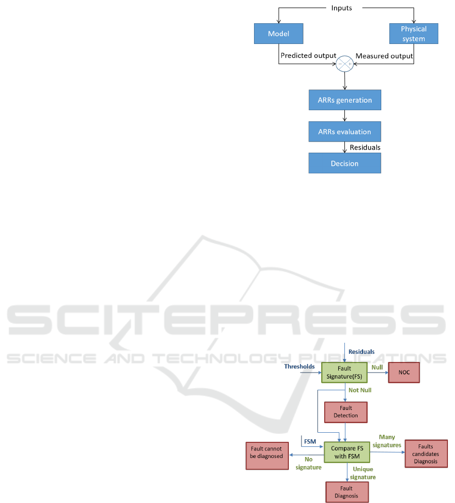
As represented in Figure 1, the ﬁrst step of a

model-based FDD procedure consists of comparing

the system’s available measurements (measured out-

put) with a priori information represented by the sys-

tem’s mathematical model (predicted output). This is

known as Analytical Redundancy Relations (ARRs)

generation. These ARRs are speciﬁc constraints rep-

resented as algebraic differential equations that con-

tain only known variables (measured outputs, system

parameters and inputs). The numerical evaluation of

the ARRs at every time instant produces a set of resid-

uals r

, expressed as follows:

= Θ(y

, u

, ρ) (1)

where k is the time instance, y

are the measured

outputs, u

the input signals, ρ the system parameters

Figure 1: Principle of model-based FDD.

and Θ is a function deduced from the residual gen-

erator method chosen for the FDD (observer, parity

relations, etc.)

In order to take a decision about the system being

in a normal or in a faulty state, the set of residuals

are compared, at each time instance k, against ﬁxed

or adaptive threshold (See Figure 2). These latter are

determined using different methods. One can cite sta-

tistical monitoring schemes (such as traditional She-

whart control charts (Areepong, 2013)), or set-based

methods that consider the noise effect and model un-

certainty (Chatti et al., 2016).

Figure 2: Model-based FDD decision.

The residuals comparison against thresholds pro-

duces a set of fault signatures (FS):

FS(k) = [FS

(k), FS

(k), ..., FS

(k)] where:

(k) =



1 if r

overcomes the associated thresholds

0 otherwise

Accordingly, if the FS is null, the system is in

Normal Operating Conditions (NOC). Otherwise, an

undesired behavior is occurring in the system.

ICINCO 2019 - 16th International Conference on Informatics in Control, Automation and Robotics

The fault isolation is then performed by compar-

ing the FS with a speciﬁc binary matrix called the

Fault Signature Matrix (FSM), which links theoreti-

cally the residuals sensitivity to the potential faults.

The columns of this matrix represent the set of resid-

uals while its rows are related to the faults. The matrix

elements are determined as follows:

i j



1 if residual i is sensitive to fault j

0 otherwise

Hence, when a FS is unique, the fault can be de-

tected and isolated. Otherwise, the obtained FS can

lead to an insufﬁcient result, i.e. the fault can be only

detected.

2.2 Limits and Challenges

The overview on the model-based diagnosis method-

ology highlights a number of challenges that may be

tackled:

• In order to determine the faults that can be de-

tected and isolated by the model-based method,

a theoretical FSM should be built. The classical

way for building a FSM considers that all the el-

ements appearing in the residual’s expression are

associated with faults. Hence, the set of faults that

can be detected and isolated is deﬁned solely by

the constitutive elements of the generated residu-

als. This represents a clear limitation since a fault

that cannot be expressed in the residual expres-

sion cannot be detected and isolated. Therefore,

unidentiﬁed faults whose origin remains undeter-

mined are not tackled by classical model-based

approaches.

• The theoretical FSM links the residuals to the po-

tential faults. These faults must have a physical

meaning representing either faults that are associ-

ated with components involved in the modeling of

the system, or faults on physical phenomena oc-

curring in the process. This reduces the scope of

model-based approaches, since the origin of faults

can be be explained by other phenomena such as

correlations for example.

• Finally, the classical FSM is completely con-

structed in a theoretical way and does not exploit

the historical faulty data that can be available.

Only Normal operating data is used to validate

the proposed model, and to compute the thresh-

old values.

The purpose of this work is to perform a deeper

and an experimental faults-to-residuals correlation

study through the exploitation of a physical model as

well as historical data, whether it belongs to the nor-

mal operating state or the faulty states. Indeed, mod-

ern systems are increasingly automated and hence,

they allow the access to a signiﬁcant amount of data.

Therefore, an experimental approach, called Fault

Training Analysis (FTrA), is presented in the follow-

ing. It can determine the causal relations between

residuals and faults that already occurred in the sys-

tem, by dealing with real measurement data, leading

to the construction of an experimental FSM that can

enhance the theoretical one. Therefore, many chal-

lenges aforementioned are raised.

3 FAULT TRAINING ANALYSIS

In this section, the FTrA is detailed and the construc-

tion of the FTrM is addressed.

3.1 Fault Training Analysis

First, we assume the following hypothesis:

Hypothesis 1. A model can be developed for the sys-

tem to be monitored.

From this available model that describes the sys-

tem’s behavior, a set of residuals r = [r

, r

, ..., r

generated by applying a model-based FDD approach,

is deﬁned.

Second, the following hypothesis are admitted:

Hypothesis 2. All sensors are faults free.

Hypothesis 3. Training data sets are available.

Hence, a set of classes C = {NOC, D

, ..., D

}

that represent all the system’s states is introduced,

where NOC is the normal operating conditions and

D = {D

, ..., D

} is a set of faults that may occur in

the system. These faults are identiﬁed in the training

data sets and can affect the actuators as well as the

sensors or the plant.

The idea behind the FTrA is to determine the

potential links between the residuals generated on

the basis of a model and the faults training data sets

available on the system. This can be done through a

FTrM, constructed during the training phase.

Deﬁnition 1. A Fault Training Matrix is an exper-

imental FSM that evaluates each generated residual

with the available faulty training data sets in order to

Fault Training Matrix for Process Monitoring based on Structured Residuals

link residuals to potential faults, with speciﬁc thresh-

olds for each of them. The columns of this matrix rep-

resent the set of residuals while its rows are related to

the faults identiﬁed in the training data sets.

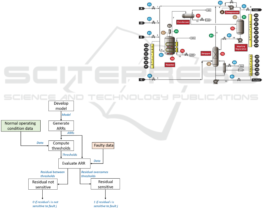
3.2 Fault Training Matrix

The FTrM construction procedure is given in Figure

3 and detailed as follows:

1. Develop the physical/graphical model describing

the system behavior.

2. Generate ARRs.

3. Compute thresholds for each ARR, using histor-

ical data from normal operating conditions. This

step can be addressed by various approaches as

aforementioned.

4. For each fault scenario, use the faulty observa-

tions (data) to numerically evaluate each ARR:

• if the residual overcomes its associated thresh-

olds then it is assumed that the residual is sen-

sitive to the considered fault scenario.

• if the residual remains between its associated

thresholds then it is assumed that the residual is

not sensitive to the considered fault scenario.

5. Determine the FTrM elements as follows:

i j



1 if residual i is sensitive to fault j

0 otherwise

Figure 3: FTrM construction principle.

The FTrM is then used on-line to detect and iso-

late faults that may occur in the system, following the

same reasoning in Figure 2.

4 APPLICATION

In this section, the classical model-based FDD ap-

proach as well as the proposed Fault Training Analy-

sis are applied on the well-known Tennessee Eastman

Process. A critical discussion and a comparison are

given.

4.1 The TEP

The Tennessee Eastman Process (TEP) is a realistic

industrial benchmark that consists of ﬁve units: a re-

actor, a condenser, a compressor, a separator and a

stripper (Downs and Vogel, 1993). The process ﬂow

sheet of the TEP is presented in Figure 4.

Figure 4: Process ﬂow sheet of the TEP.

The reactants A, D, E, C (corresponding respec-

tively to Streams 1; 2;3;4) are introduced into the re-

actor to form the liquid products G, H and a byproduct

It is worth noting that 41 process measurements

are available, as well as 12 input variables. More de-

tails are given in (Downs and Vogel, 1993).

Many researchers and practitioners evaluated and

compared their monitoring approaches on the TEP

(Verron et al., 2010), (Atoui et al., 2016), (Ghosh

et al., 2011), (Ding et al., 2009), (Yin et al., 2012)

since this benchmark can simulate different faults, de-

tailed in Table 1. Indeed, training and test data sets

are generated from the TEP by recording the process

measurements under NOC and the aforementioned

faults.

4.2 Classical Model-based FDD

In this section, a classical model-based approach is

applied for the FDD of the TEP. This approach relies

on a BG model that has been previously developed

by the authors in (Tidriri et al., 2018).

ICINCO 2019 - 16th International Conference on Informatics in Control, Automation and Robotics

Table 1: Process faults.

Fault Description Type

A/C feed ratio, B composition constant (Stream 4) step

B composition, A/C ratio constant (Stream 4) step

Condenser cooling water inlet temperature step

A feed loss (Stream 1) step

C header pressure loss-reduced availability (Stream 4) step

A, B, and C feed composition (Stream 4) random

Condenser cooling water inlet temperature random

Reaction kinetics drift

The BG model of a part of the TEP (the reactant

A) is given as an example in Figure 5.

The BG model of the TEP is then used to gener-

ate residuals. This is done by adopting the strategy

of eliminating unknown variable by substituting them

using only measured and known ones. Details about

this procedure can be found in (Chatti et al., 2014),

(Tidriri et al., 2018).

18 residuals were generated for the TEP. For the

sake of clarity, only 4 residuals expressions, in the

steady state, are given in the following:

= y

+ y

−C

dµ

−

− y

(2)

= y

−C

dµ

−

∑

j=1

A j

−C

dµ

− y

+ F

) − x

A10

(3)

= y

+ y

−C

dµ

−

− y

(4)

= y

−C

dµ

−

∑

j=1

b j

−C

dµ

− y

+ F

) − x

B10

= 0 (5)

The classical model-based approach relies on the

fact that residuals expression deﬁne the set of de-

tectable and isolable faults. Therefore, according to

the expression of residuals r

and r

related to gas A

for example, the detectable faults involve the chemi-

cal potentials (µ

, µ

), the sensors which measure

several ﬂows (A feed ﬂow F

, overhead ﬂow from

the stripper F

, recycled ﬂow F

, reactor feed rate F

purge rate F

, the product separator underﬂow F

, the

reaction kinetics through the reaction rate τ

, the fric-

tions in the mixing and the reactor zone (R

, R

) and

the potential energy stored in the mixing, reactor and

separator zones (C

, C

In order to exploit the available historical data, the

FTrA is performed in the following.

4.3 Fault Training Analysis of the TEP

In this step, known variables of the TEP are used in

normal operating conditions (NOC) and faulty states,

in order to determine which residuals react in pres-

ence of different faults. Hence, all obtained residu-

als are evaluated with available measured outputs and

control inputs.

For example, residual r

was evaluated us-

ing known variables that appear in its expres-

sion, namely (F

, F

) for each faulty scenario

, D

, ..., D

). If the residual is sensitive to a faulty

scenario, its column value in the FTrM will be equal

to 1. It appeared that residual r

reacts and exceeds

its ﬁxed thresholds in presence of measurements from

6 faulty scenarios: (D

, D

). Hence,

these faults have an impact on the measured outputs

and control inputs within sensors free-fault case. Ac-

cordingly, a 1 is added in the FTrM, for each corre-

sponding fault, as shown in Table 2.

The same reasoning is applied for the remaining

residuals.

During this testing campaign, we noted that 3

residuals (r

, r

) did not react to any faulty sce-

nario. Therefore, they are not considered in the FTrM.

Furthermore, it appears that it is possible to isolate

all faults affecting the TEP using a subset of residuals.

Hence, a mutual information based algorithm (Verron

et al., 2008) is applied to obtain a reduced subset of 5

residuals with unique FS (r

, r

The Fault Signature (FS) is then represented by the

following vector of 5 residuals (r

, r

The deduced reduced FTrM (Table 3) is used in

the on-line monitoring strategy of the TEP, as de-

scribed previously in Figure 2.

Fault Training Matrix for Process Monitoring based on Structured Residuals

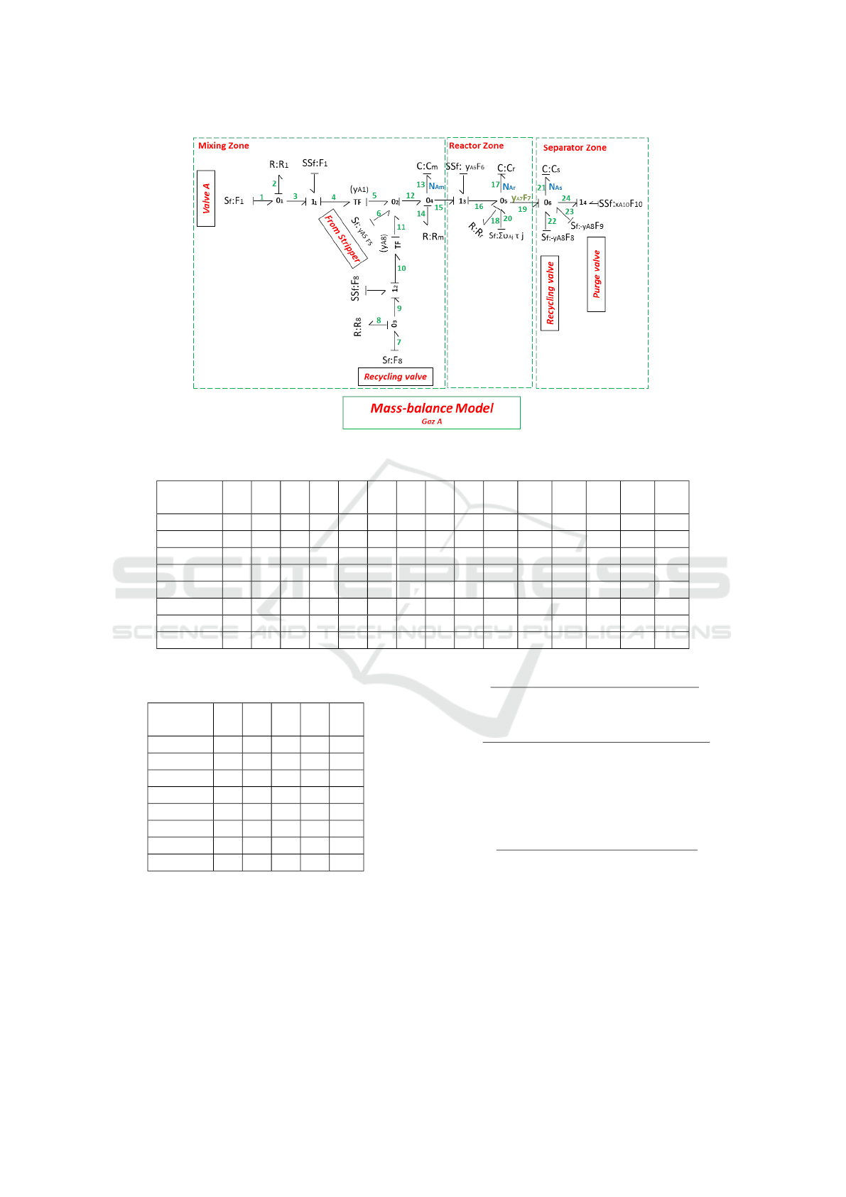
Figure 5: Mass-balance BG of reactant A in the TEP, with derivative causality.

Table 2: Fault Training Matrix (FTrM) linking faults to residuals.

1 0 1 0 0 0 0 0 0 0 0 0 0 0 0

0 1 0 1 0 1 0 1 1 0 1 1 1 1 1

0 0 1 0 0 0 0 0 1 0 1 0 0 0 0

1 0 0 0 0 0 0 0 1 0 1 0 0 0 0

1 1 1 0 1 1 0 1 1 1 1 0 0 0 0

1 0 1 0 0 0 0 0 1 0 1 0 0 0 0

1 1 0 0 1 1 0 1 1 0 1 0 0 0 0

1 1 1 1 1 1 1 1 1 0 1 0 0 0 0

Table 3: Reduced Fault Training Matrix (FTrM) linking

faults to residuals.

1 1 0 0 0

0 0 1 1 1

0 1 0 0 1

1 0 0 0 1

1 1 0 1 1

1 1 0 0 1

1 0 0 1 1

1 1 1 1 1

4.4 Results and Comparison

Detection performances are evaluated using the false

alarm rate (FAR), which is the percentage of normal

samples identiﬁed as fault (See (6)), and fault detec-

tion rate (FdR), which is the percentage of samples

correctly detected (See (7)).

FAR =

No. of normal samples identiﬁed as fault

Total No. of normal samples

∗ 100

(6)

FdR =

No. of faulty samples correctly detected

Total No. of faulty samples

∗100

(7)

As for diagnosis performances, they are evaluated

using the fault diagnosis rate (FDR):

FDR =

No. of samples correctly diagnosed

Total No. of samples

∗ 100

(8)

The results are given in Tables 4 and 5. A com-

parison between many works reported in the litera-

ture (Fisher Discriminant Analysis (FDA) (Yin et al.,

2012), Principal Component Analysis (PCA) (Yin

et al., 2012), (Ghosh et al., 2014), Partial Least

Squares (PLS) (Yin et al., 2012), Dynamic PCA

(DPCA) (Yin et al., 2012), Bayesian Network (BN)

(Verron, 2007), Independant Component Analysis

(ICA) (Yin et al., 2012), Simple Neural Network

ICINCO 2019 - 16th International Conference on Informatics in Control, Automation and Robotics

Table 4: Comparison of fault detection performance (%) for the TEP, with reduced FTrM.

FDA PCA PLS PCA DPCA BN ICA BG

Average FdR 79.13 90.60 90.82 90.86 92.39 98.92 98.95 99.94

FAR 3.11 6.13 10 1.56 10.13 1.13 2.75 0.38

Table 5: Comparison of fault diagnosis performance (%) for the TEP, with reduced FTrM.

SNN SVM PCA NN BN BG

Average FDR 60.63 62.77 74.82 79.13 95.78 88.66

(SNN) (Eslamloueyan, 2011), Support Vector Ma-

chine (SVM) (Jing and Hou, 2015), PCA (Jing and

Hou, 2015), NN (Eslamloueyan, 2011), BN (Verron,

2007)), based solely on data, and the proposed en-

hanced BG approach is addressed.

The absence of model-based approaches within this

comparison is due to the fact that no work has at-

tempted to detect and diagnose the faults affecting the

TEP by using a model. The red color indicates the

best result.

According to Table 4, it appears that the pro-

posed BG approach presents the best detection per-

formances. Indeed, it has the highest FdR (99.94%).

6 faults are perfectly detected (D

, D

)

in 100% of the observations. Furthermore, the BG ap-

proach shows the lowest FAR (0.38%).

Thus, the proposed BG approach shows the best FAR

and FdR.

Regarding the diagnosis performances, the pro-

posed BG approach shows the second best perfor-

mance, with an average FDR of 88.66%, as indicated

in Table 4.

Accordingly, the BG approach, enhanced with the

FTrA, presents better or comparable performances

than many data-driven methods reported in the litera-

ture.

5 CONCLUSION

In this work, an enhanced model-based approach was

proposed for fault detection and diagnosis of a well-

known industrial benchmark: the Tennessee Eastman

process.

The proposed approach improves the classical

fault detection and diagnosis model-based scheme by

extending it to an experimental approach, i.e. the

Fault Training Analysis, that exploits the available

historical data from nominal as well as faulty states.

The purpose of this latter is to identify the causal re-

lationships between residuals and faults. The fault

training analysis results on an experimental matrix,

called Fault Training Matrix, that enhances the theo-

retical Fault Signature Matrix.

The proposed approach was validated through the

Tennessee Eastman Process, and shows a high fault

detection rate, a high fault diagnosis rate and a small

false alarm rate.

REFERENCES

Areepong, Y. (2013). A comparison of performance of

residual control charts for trend stationary processes.

International Journal of Pure and Applied Mathemat-

ics, 85(3):583–592.

Atoui, M. A., Verron, S., and Kobi, A. (2016). A bayesian

network dealing with measurements and residuals for

system monitoring. Transactions of the Institute of

Measurement and Control, 38(4):373–384.

Chatti, N., Guyonneau, R., Hardouin, L., Verron, S.,

and Lagrange, S. (2016). Model-based approach

for fault diagnosis using set-membership formula-

tion. Engineering Applications of Artiﬁcial Intelli-

gence, 55:307–319.

Chatti, N., Ould-Bouamama, B., Gehin, A.-L., and Mer-

zouki, R. (2014). Signed bond graph for multiple

faults diagnosis. Engineering Applications of Artiﬁ-

cial Intelligence, 36:134–147.

Ding, S. (2008). Model-based fault diagnosis techniques:

design schemes, algorithms, and tools. Springer Sci-

ence & Business Media.

Ding, S. X., Zhang, P., Naik, A., Ding, E. L., and Huang,

B. (2009). Subspace method aided data-driven design

of fault detection and isolation systems. Journal of

process control, 19(9):1496–1510.

Downs, J. J. and Vogel, E. F. (1993). A plant-wide indus-

trial process control problem. Computers & chemical

engineering, 17(3):245–255.

Eslamloueyan, R. (2011). Designing a hierarchical neural

network based on fuzzy clustering for fault diagnosis

of the tennessee–eastman process. Applied soft com-

puting, 11(1):1407–1415.

Gao, Z., Cecati, C., and Ding, S. X. (2015). A survey

of fault diagnosis and fault-tolerant techniques—part

i: Fault diagnosis with model-based and signal-based

approaches. IEEE Transactions on Industrial Elec-

tronics, 62(6):3757–3767.

Ghosh, K., Ng, Y. S., and Srinivasan, R. (2011). Evaluation

of decision fusion strategies for effective collaboration

among heterogeneous fault diagnostic methods. Com-

puters & chemical engineering, 35(2):342–355.

Fault Training Matrix for Process Monitoring based on Structured Residuals

Ghosh, K., Ramteke, M., and Srinivasan, R. (2014). Op-

timal variable selection for effective statistical pro-

cess monitoring. Computers & Chemical Engineer-

ing, 60:260–276.

Isermann, R. (2005). Model-based fault-detection and di-

agnosis–status and applications. Annual Reviews in

control, 29(1):71–85.

Jha, M. S., Chatti, N., and Declerck, P. (2017). Robust

fault detection in bond graph framework using interval

analysis and fourier-motzkin elimination technique.

Mechanical Systems and Signal Processing, 93:494–

514.

Jing, C. and Hou, J. (2015). Svm and pca based fault clas-

siﬁcation approaches for complicated industrial pro-

cess. Neurocomputing, 167:636–642.

Liu, J., Luo, W., Yang, X., and Wu, L. (2016). Robust

model-based fault diagnosis for pem fuel cell air-feed

system. IEEE Transactions on Industrial Electronics,

63(5):3261–3270.

Sidhu, A., Izadian, A., and Anwar, S. (2015). Adaptive

nonlinear model-based fault diagnosis of li-ion bat-

teries. IEEE Transactions on Industrial Electronics,

62(2):1002–1011.

Tidriri, K., Chatti, N., Verron, S., and Tiplica, T. (2016).

Bridging data-driven and model-based approaches for

process fault diagnosis and health monitoring: A re-

view of researches and future challenges. Annual Re-

views in Control.

Tidriri, K., Chatti, N., Verron, S., and Tiplica, T. (2018).

Model-based fault detection and diagnosis of complex

chemical processes: A case study of the tennessee

eastman process. Proceedings of the Institution of

Mechanical Engineers, Part I: Journal of Systems and

Control Engineering, page 0959651818764510.

Verron, S. (2007). Diagnostic et surveillance des processus

complexes par r

eseaux bay

esiens. PhD thesis, Univer-

sit

e d’Angers.

Verron, S., Li, J., and Tiplica, T. (2010). Fault detec-

tion and isolation of faults in a multivariate process

with bayesian network. Journal of Process Control,

20(8):902–911.

Verron, S., Tiplica, T., and Kobi, A. (2008). Fault detection

and identiﬁcation with a new feature selection based

on mutual information. Journal of Process Control,

18(5):479–490.

Yang, Y., Ding, S. X., and Li, L. (2015). On observer-based

fault detection for nonlinear systems. Systems & Con-

trol Letters, 82:18–25.

Yin, S., Ding, S. X., Haghani, A., Hao, H., and Zhang,

P. (2012). A comparison study of basic data-driven

fault diagnosis and process monitoring methods on

the benchmark tennessee eastman process. Journal

of Process Control, 22(9):1567–1581.

Zhong, M., Song, Y., and Ding, S. X. (2015). Parity space-

based fault detection for linear discrete time-varying

systems with unknown input. Automatica, 59:120–

126.

ICINCO 2019 - 16th International Conference on Informatics in Control, Automation and Robotics