Investigation on Viscoelastic Fluid Behavior by Modifying Deviatoric
Stress Tensor
Nobuhiko Mukai, Erika Matsui and Youngha Chang
Computer Science, Tokyo City University, 1-28-1 Tamazutsumi, Setagaya, Tokyo, Japan
Keywords:
Particle Method, Viscoelastic Fluid, Spinnability, Cauchy’s Equation of Motion, Deviatoric Stress.
Abstract:
One of the most challenging issues is to simulate and visualize liquid behavior, especially viscoelastic fluid,
which has both characteristics of viscosity and elasticity. Although Newtonian fluid, which is represented by
water, is generally analyzed with the governing equations, which are Navier-Stokes equation and equation
of continuity. However, viscoelastic behavior is so complex that there is no established governing equation
such as Newton’s equation of motion and Navier-Stokes equation. Some researchers employ Finite Element
Method and others develop their own point based methods. In addition, there is a characteristic feature called
“Spinnability” in viscoelastic fluid. That is, viscoelastic fluid is stretched so long and shows sudden shrink
when the stretched fluid is broken. Then, we have been performing this spinnability simulation based on
Cauchy’s equation of motion by modifying the stress term in constitutive equation. In this paper, we report
the simulation results on viscoelastic fluid behavior for four kinds of deviatoric stress tensors constructing
Cauchy’s equation of motion: only viscosity, only elasticity, linear combination of viscosity and elasticity, and
complex modulus of elasticity.
1 INTRODUCTION
Nowadays, computer graphics can present almost ev-
erything from artificial objects to natural phenomena
such as buildings, cars, robots, lighting, snowstorm,
aurora and so on. Among these things, one of the
most difficult and challenging tasks is to simulate and
visualize liquid behavior since its deforms so dynam-
ically yet the boundary of it is very clear, while solid
body does not deform so largely, and the boundary
of gas is not clear. In the liquid simulation, Newto-
nian fluid represented by water is comparatively sim-
ple to be simulated since the relation between shear-
ing stress and velocity gradient is linear.
In the world, there are many non-Newtonian flu-
ids, and one of them is called “viscoelastic fluid”,
which has both features of viscosity and elasticity, and
the relation between shearing stress and velocity gra-
dient is not linear. The behavior is so complicated that
many researchers have tried to simulate and visual-
ize the behavior of viscoelastic fluid. However, there
is no established governing equation for viscoelastic
fluid. Some researchers employ FEM (Finite Element
Method) and SM (Spring Mass) model to visualize
the deformation, and others are developing various
kinds of methods, which are based on point method.
Moreover, there are some works based on Navier-
Stokes equation, which is the established governing
equation of fluid. These researches are trying to sim-
ulate the viscoelastic fluid behavior by adding viscous
and elastic stress terms as the external force.
In addition, viscoelastic fluid has the characteris-
tic feature called “spinnability”. Viscoelasic fluid can
be stretched so long as if it is a string and shrinks
suddenly when it is broken. This is “spinnability”,
and there are some works on spinnability; however,
almost all of them do not quote the word of spinnabil-
ity and just simulate that viscoelastic fluid is stretched
so long like a string.
Then, we have been trying to simulate this char-
acteristic feature of viscoelastic fluid on the basis of
Cauchy’s equation of motion, which is the basic equa-
tion of motion for continuum. In Cauchy’s equation
of motion, there is a term of “deviatoric stress”, and
we think that this stress term should have both char-
acteristics of viscosity and elasticity, and have been
trying to simulate the behavior and to measure the
stretched length by replacing this term with a linear
combination of viscous and elastic terms.
In this paper, we re-investigate the liner combina-
tion of the deviatoric stress term, and consider only
viscosity term or only elasticity term for the simula-
216
Mukai, N., Matsui, E. and Chang, Y.
Investigation on Viscoelastic Fluid Behavior by Modifying Deviatoric Stress Tensor.
DOI: 10.5220/0007788702160222
In Proceedings of the 9th International Conference on Simulation and Modeling Methodologies, Technologies and Applications (SIMULTECH 2019), pages 216-222
ISBN: 978-989-758-381-0
Copyright
c
 2019 by SCITEPRESS – Science and Technology Publications, Lda. All rights reserved

tion. In addition, we consider complex modulus of
elasticity, which can handle both viscosity and elas-
ticity in one term with complex number. This paper
describes the method of the simulations with four dif-
ferent deviatoric stress terms, and shows the results of
the simulations.
2 RELATED WORKS
Related to works on Newtonian fluid represented by
water, (Mould and Yang, 1997) surveyed about wa-
ter modeling and showed that there were two types of
studies: hydrodynamic theory based research and ex-
perimental based works. (Iglesias, 2004) also inves-
tigated papers published during the 1980s and 1990s.
In addition, (Darles et al., 2011) published a survey on
computer graphics based ocean simulation and ren-
dering. According to the survey, there are two types
of researches. One is a physics based method using
Navier-Stokes equation, and the other is an empirical
law based oceanographic work.
(Hinsinger et al., 2002), (Cui et al., 2004) and
(Dupuy and Bruneton, 2012) employed mesh mod-
eling to represent ocean waves, irregular long crest
waves, and vast ocean scene, respectively since ocean
waves basically have continuous surfaces. How-
ever, as the drawbacks, re-meshing is required ev-
erytime the topology changes. On the other hand,
(M¨uller et al., 2003) and (Kipfer and Westermann,
2006) utilized SPH (Smoothed Particle Hydrodynam-
ics), which is one of particle methods, for solving
Navier-Stokes equation with surface tension. They
presented water pouring into a glass and river flow-
ing from a rock, respectively.
In relation to the simulation of fluid behavior, two
kinds of methods are usually used. One is an Eu-
lerian (grid based) method and the other is a La-
grangian (particle based) method. (Chentanez and
M¨uller, 2011) and (Nishino et al., 2012) utilized Eu-
lerian simulation methods to propose an optimized
grid for GPU (Graphics Processing Unit) and to rep-
resent freezing ice with air bubbles, respectively. On
the other hand, (Foster and Fedkiw, 2001) employed
semi-Lagrangian method to represent viscous liquids
interacting with 3D objects and (Busaryev et al.,
2012) proposed a particle based algorithm to repre-
sent bubbles with Voronoi diagram.
Moreover, there is a hybrid method of Eulerian
and Lagrangian methods. (Hong et al., 2008) and
(Chentanez and M¨uller, 2010) used the hybrid method
to represent bubbles in water and spray or splash, re-
spectively. (Miller, 1989) also proposed a method to
animate viscous fluid with collision between particles
and obstacles, and (Sims, 1990) developed a parallel
particle rendering system that allows to treat particles
with different shapes, sizes, colors and transparen-
cies. In addition, (Greenwood and House, 2004) and
(Geiger et al., 2006) proposed particle level-set algo-
rithms to visualize various kinds of bubble shapes and
fine splash particles, respectively. In addition, (Kim
et al., 2007) adopted a levelset method to present bub-
bles in liquid and gas interaction, and (Losasso et al.,
2008) also used a particle level set method for dense
liquid volume and utilized a particle method for dif-
fused regions.
As mentioned above, there are some basic types
for the simulation of Newtonian fluid such as water.
One is a Eulerian (grid based) method and the other is
a Lagrangian (particle based) method, although mesh
modeling is included in grid based modeling and par-
ticle level set method is part of particle based meth-
ods. Of course, some researches are based on exper-
imental observations, and others obey Navier-stokes
equation. However, experimental observations de-
pend on the environment when the data are obtained.
Then, Navier-Stokes equation should be used for the
stable and precise fluid simulation as Newton’s equa-
tion of motion is used for solid mechanics.
Now, for the previous works on the simulation of
viscoelastic fluid, (Tamura et al., 2005) used spring-
mass system to visualize an egg dropping on the floor.
In addition, (Bargteil et al., 2007) and (Wojtan and
Turk, 2008) employed Finite Element methods to rep-
resent large plastic deformation of solid materials and
to simulate the complex elastic and plastic behavior
of viscoelastic materials, respectively. These methods
are in the group of Eulerian methods. On the other
hand, (Clavet et al., 2005) employed a particle based
method for viscoelastic fluid simulation; however, the
method also added springs to accomplish elastic and
non-linear plastic effects. (Ram et al., 2015) proposed
a new method called “Material Point Method” to sim-
ulate foams and sponges, and employed Oldroyd-B
model to preserve plastic volume. (Barreiro et al.,
2017) developeda constrained dynamics solver by ex-
tending position based dynamics method to represent
whipped cream and strawberry syrup. These methods
are some kinds of particle methods or hybrid methods.
They do not obey Navier-Stokes equation as the gov-
erning equation although some works employ conser-
vation of mass and momentum.
(Goktekin et al., 2004) used a grid based method
with level set to animate viscoelastic fluids such as
mucus, liquid soap and so on. On the other hand,
(Chang et al., 2009) utilized a particle based method
called SPH (Smoothed Particle Hydrodynamics) to
visualize melting and flowing viscoelastic fluid. Al-
Investigation on Viscoelastic Fluid Behavior by Modifying Deviatoric Stress Tensor
217

though these studies used different methods, they
both employed Navier-Stokes equation as the govern-
ing equation of viscoelastic fluid because viscoleas-
tic fluid also has characteristics of fluid and Navier-
Stokes equation is the established governing equation
to analyze fluid behavior. In addition, they both added
viscosity and elasticity terms to Navier-Stokes equa-
tion as the external term.
Navier-stokes equation is the established govern-
ing equation of fluid, and viscoelastic fluid has both
characteristic features of viscosity and elasticity. Vis-
cosity is a feature of fluid, while elasticity is an-
other feature of elastic body that is a kind of con-
tinuum. Then, the governing equation of viscoelastic
fluid should be Cauchy’s equation of motion, which is
the governing equation of continuum as if Newton’s
equation of motion is the governing equation for solid
mechanics. Cauchy’s equation of motion has a term
of “deviatoric stress”, which should have both charac-
teristic of viscosity and elasticity. Then, (Mukai et al.,
2010) and (Mukai et al., 2018) have tried to simu-
late viscoelastic fluid behavior by introducing a linear
combination of viscosity and elasticity terms for the
deviatoric term of Cauchy’s equation of motion, and
to evaluate the length of the viscoelastic fluid when it
is stretched.
In this paper, we re-investigate the linear combi-
nation between viscous and elastic terms of the devi-
atoric stress, and evaluate the behavior of viscoelas-
tic fluid by considering three new terms: only viscos-
ity term, only elasticity term and complex modulus of
elasticity that can handle both features in one term.
3 METHOD
We employ MPS (Moving Particle Semi-implicit)
method for the simulations. MPS is one of particle
methods and was developed for incompressible fluid.
In the research, the governing equations are equation
of continuity and Cauchy’s equation of motion de-
scribed as follows.
Equation of continuity:
dρ
dt
= 0 (1)
Cauchy’s equation of motion with surface tension:
ρ
dv
v
v
dt
= ∇·σ
σ
σ+ g
g
g+ f
f
f = (−∇pI
I
I + ∇ · τ
τ
τ) + g
g
g+ f
f
f (2)
where, ρ is density, t is time, v
v
v is velocity, σ
σ
σ is stress
tensor, g
g
g is the gravity, f
f
f is external force, p is pres-
sure, I
I
I is unit matrix, and τ
τ
τ is deviatoric stress.
The target is viscoelastic fluid that has both fea-
tures of viscosity and elasticity. Then, τ
τ
τ should have
both features and can be written as the following.
τ
τ
τ = ατ
τ
τ
v
+ (1− α)τ
τ
τ
e
(3)
τ
τ
τ
v
= 2η
0
D
D
D (4)
D
D
D =
1
2
(L
L
L+ L
L
L
t
), L
L
L = ∇V
V
V (5)
V
V
V = (u
u
u,v
v
v,w
w
w) (6)
∇V
V
V =



∂u
u
u
∂x
∂u
u
u
∂y
∂u
u
u
∂z
∂v
v
v
∂x
∂v
v
v
∂y
∂v
v
v
∂z
∂w
w
w
∂x
∂w
w
w
∂y
∂w
w
w
∂z



(7)
τ
τ
τ
e
= 2µε
ε
ε, µ =
E
2(1+ ν)
(8)
where, τ
τ
τ
v
and τ
τ
τ
e
are viscosity and elasticity terms of
deviatoric stress, respectively, and α is a linear com-
bination coefficient. η
0
is zero shear viscosity, V
V
V is
velocity, ε
ε
ε is distortion tensor, E is Young’s modulus
and ν is Poisson’s ratio.
α is defined as follows by approximating the fig-
ure showing the relation between shearing velocity
and viscosity researched by (Isogai, 2008) and by nor-
malizing so that the maximum value becomes 1.0. In
Eq.(4), there is an assumption that the volume of the
viscoelactic fluid does not change.
α = 4.99 × 10
−4
˙
γ
2
− 3.07× 10
−2
˙
γ+ 1 (9)
where,
˙
γ is shearing velocity, which is calculated as
follows.
˙
γ =
p
2II
D
(10)
II
D
=
1
2
(D
ii
D
j j
− D
ij
D
ji
) (11)
=
1
2
(D
11
D
22
+ D
22
D
33
+ D
33
D
11
−D
12
D
21
− D
23
D
32
− D
31
D
13
) (12)
where, D
ij
is the ith row jth column element of D
D
D,
and II
D
is called the second invariant of deformation
velocity tensor.
Here, as the external force f
f
f in Eq.(2), we con-
sider the surface tension. In fact, there are two types
of models for the surface tension. One is CSF (Con-
tinuum Surface Force) model, which is calculated
with the shape of the free surface, and the other is
a potential model, which is calculated by considering
potential energy of each particle. CSF model is pop-
ular and is widely used; however, it is not stable in
case there are not enough free surface particles. Then,
we adopt a potential model proposed by (Koshizuka,
2014) to calculate the surface tension.
The following potential force P(r
ij
) works be-
tween particles i and j, and the surface tension f
f
f is
calculated with the potential coefficientC
p
as follows.
SIMULTECH 2019 - 9th International Conference on Simulation and Modeling Methodologies, Technologies and Applications
218

P(r
ij
) =

1
3
C
p
(r
ij
−
3
2
l
0
+
1
2
r
e
)(r
ij
− r
e
)
2
(r
ij
≤ r
e
)
0 otherwise
(13)
f
f
f = Σ
j6=i
{C
p
(r
ij
−l
0
)(r
ij
−r
e
)(r
r
r
j
−r
r
r
i
)/r
ij
}
(14)
where, r
r
r
i
and r
r
r
j
are the positions of particles i and
j, r
ij
is the distance between particles i and j, l
0
is
initial distance between particles, and r
e
is radius of
influence. C
p
is calculated from the wetting angle be-
tween the fluid and the solid contacted by the fluid.
In addition, we consider complex modulusof elas-
ticity that handles both viscosity and elasticity in one
term with complex number. Complex modulus of
elasticity E
∗
(ω) is written as follows.
E
∗
(ω) =

1
E
+
1
i
u
ωη

−1
(15)
where, E is Young’s modulus, i
u
is imaginary unit, ω
is angular velocity, η is viscosity coefficient.
Then, the deviatoric stress is calculated with the
complex modulus of elasticity as the following.
τ
τ
τ = E
∗
(ω)ε (16)
=

E + i
u
ωη
i
u
Eωη

−1
ε (17)
=

i
u
Eωη
E + i
u
ωη

ε (18)
=
E(ωη)
2
+ i
u
E
2
ωη
E
2
+ (ωη)
2
ε (19)
|τ
τ
τ| = ε
s

E(ωη)
2
(ωη)
2
+ E
2

2
+

E
2
(ωη)
(ωη)
2
+ E
2

2
(20)
Here, η in the above equations is also calculated
as follows by approximating the figure showing the
relation between shearing velocity and viscosity (Iso-
gai, 2008); however it is not normalized as in Eq.(9)
because this value is not a coefficient.
η = 1.80 × 10
−4
˙
γ
2
− 1.11× 10
−2
˙
γ+ 3.62× 10
−1
(21)
4 SIMULATION
Table 1 and 2 show the specification of the PC and the
parameters used for the simulation, respectively.
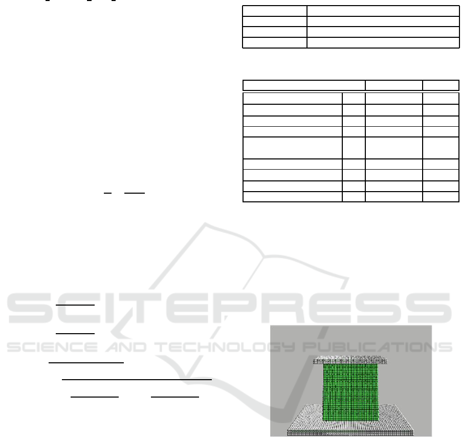
Fig.1 shows the initial position of the viscoelas-
tic fluid, which sticks to two solid bodies on both the
Table 1: PC specification.
OS Windows 7 Professional 64 bit
CPU Intel Core i5-2500K 3.3GHz
Main memory 4GB
GPU GeForce GTX 570 with 4GB memory
Table 2: Parameters used for the simulation.
Parameter Value Unit
Density ρ 1.16× 10
3
kg/m
3
Young’s modulus E 1.05× 10
3
Pa
Poisson’s ratio ν 0.5
Zero shear viscosity η
0
28 Pa· s
Initial distance of parti-
cles (= Particle radius)
l
0
3.0× 10
−3
m
Pulling velocity v
v
v 0.18 m/s
Time step △t 0.10× 10
−3
s
Wetting angle θ 30 degree
Angular velocity ω π/4 rad/s
upper and the lower sides. The initial numbers of
particles are about 30,000, 5,000 and 12,000 for the
viscoelastic fluid, the upper and the lower solid bod-
ies, respectively. In the simulation, the upper solid
body is pulled up, while the lower one is fixed. Then,
the viscoelastic fluid is stretched. The velocity to pull
the upper solid body increases according to sinusoidal
curve, and reaches the pulling velocity at 100 steps.
Figure 1: Initial position of the viscoelastic fluid.
There are four kinds of simulations for different
deviatoric stresses τ
τ
τ shown in Eq.(2).
Simulations for Different Deviatoric Stresses
Sim. 1 linear combination of viscosity and elasticity
based on Eq.(3), where α changes according to
Eq.(9).
Sim. 2 only viscosity term, where α is always 1.0 for
Eq.(3).
Sim. 3 only elasticity term, where α is always 0.0 for
Eq.(3).
Sim. 4 complex modulus of elasticity based on
Eq.(20).
Investigation on Viscoelastic Fluid Behavior by Modifying Deviatoric Stress Tensor
219

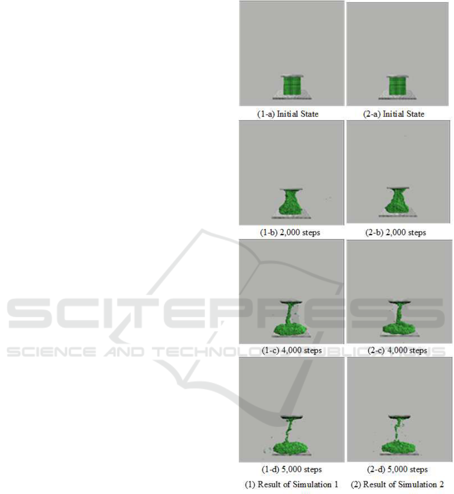
5 RESULTS
Figs.2 and 3 show the results of the simulations. Ini-
tial states are the same for all simulations; however,
the viscoelastic fluid was stretched as time went for
the simulations of 1 and 2, while particles were dis-
persed for the simulations of 3 and 4. In the simula-
tions of 1 and 2, particles have the viscosity feature
although the viscosity coefficient in the simulation 1
changes according to the shearing velocity, while the
viscosity is constant in the simulation 2. Viscosity
has the feature that puts particles together, and then
it seems that this feature prevented for particles to be
dispersed. The comparison between the simulations 1
and 2 shows that the particles in the simulation 1 are a
little bit dispersed than that in the simulation 2. On the
other hand, the simulation 3 has only elasticity feature
and does not have any viscosity feature. Then, the
particles in the simulation 3 were so dispersed. For
the simulation 4, complex modulus of elasticity was
used. This term can handle both viscosity and elas-
ticity in one term; however, the value of E is larger
than that of η so that the effect of viscosity becomes
almost zero. This is the reason why the particles in
the simulation 4 were also dispersed.
6 CONCLUSIONS
For the simulation of Newtonian fluid represented
by water, there is the established governing equation
called Navier-Stokes equation, and many studies have
been performed; however, there is no established gov-
erning equation for the simulation of non-Newtonian
fluid. Then, there are a lot of researches based on
many ideas. On the other hand, Cauchy’s equation
of motion is the established governing equation for
continuum. Then, we have been trying to simulate
spinnability of viscoelastic fluid by modifying the de-
viatoric stress, and in this paper, we have tried four
types of simulations: linear combination of viscosity
and elasticity, viscosity only, elasticity only, and com-
plex modulus of elasticity.
As the results of the simulations, the particles
were stretched without being dispersed for the sim-
ulation with linear combination of viscosity and elas-
ticity, and for the simulation with only viscosity. This
is because viscosity has the feature to put particles to-
gether. Then, if viscosity term has some effect for
the stretching, the fluid is stretched without being dis-
persed. On the other hand, if elasticity term has more
effect for the stretching, the fluid is dispersed.
Then, we have to improvethe viscosity term not to
disperse the particles; however, if viscosity has large
Figure 2: Simulation results on Sim. 1 and 2.
effect, the fluid is stretched without being broken.
Even if it is broken, it does not shrink suddenly and
does not show the characteristic feature of spinnabil-
ity. In addition, we did not consider the volume
change of the viscoelastic fluid in this paper; how-
ever, the volume might have changed because there
are not so many particles in the middle of the fluid
when it is stretched. In the future, we have to inves-
tigate how the spinnablity, which is a characteristic
feature of viscoelastic fluid, can be visualized by con-
SIMULTECH 2019 - 9th International Conference on Simulation and Modeling Methodologies, Technologies and Applications
220

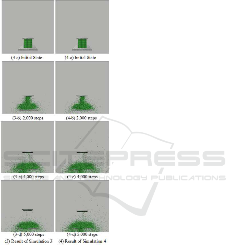
Figure 3: Simulation results on Sim. 3 and 4.
sidering the volume change of the fluid.
REFERENCES
Bargteil, A. W., Wojtan, C., Hodgins, J. K., and Turk, G.
(2007). A finite element method for animating large
viscoplastic flow. ACM Transactions on Graphics,
26(3):Article No.16.
Barreiro, H., Garc´ıa-Ferm´andez, I., Aldu´an, I., and Otaduy,
M. A. (2017). Conformation constraints for efficient
viscoelastic fluid simulation. ACM Transactions on
Graphics, 36(6):Article No.221.
Busaryev, O., Dy, T. K., Wang, H., and Ren, Z. (2012). An-
imating bubble interactions in a liquid foam. ACM
Transactions on Graphics, 31(4):63:1–63:8.
Chang, Y., Bao, K., Liu, Y., Zhu, J., and Wu, E. (2009).
A particle-based method for viscoelastic fluids anima-
tion. In Proceedings of the 16th ACM Symposiumon
Virtual Reality Software and Technology, pages 463–
468.
Chentanez, N. and M¨uller, M. (2010). Real-time simulation
of large bodies of water with small scale details. Pro-
ceedings of the 2010 ACM SIGGRAPH/Eurographics
symposium on computer animation, pages 197–206.
Chentanez, N. and M¨uller, M. (2011). Real-time eulerian
water simulation using a restricted tall cell grid. ACM
Transactions on Graphics, 30(4):82:1–82:10.
Clavet, S., Beaudoin, P., and Poulin, P. (2005). Particle-
based viscoelastic fluid simulation. In Proceedings of
the 2005 ACM SIGGRAPH/Eurographics Symposium
on Computer Animation, pages 219–228.
Cui, X., Yi-cheng, J., and Xiu-wen, L. (2004). Real-time
ocean wave in multi-channel marine simulator. Pro-
ceedings of the 2004 ACM SIGGRAPH international
conference on virtual reality continuum and its appli-
cation in industry, pages 332–335.
Darles, E., Crespin, B., Ghazanfarpour, D., and Gonzato, J.
(2011). A survey of ocean simulation and rendering
techniques in computer graphics. Computer Graphics
Forum, 30(1):43–60.
Dupuy, J. and Bruneton, E. (2012). Real-time animation
and rendering of ocean whitecaps. Proceedings of the
SIGGRAPH Asia 2012 Technical Briefs, page Article
No.15.
Foster, N. and Fedkiw, R. (2001). Practical animation of
liquids. Proceedings of the ACM SIGGRAPH 2001,
pages 23–30.
Geiger, W., Leo, M., Rasmussen, N., Losasso, F., and Fed-
kiw, R. (2006). So real it’ll make you wet. Proceed-
ings of the 2006 ACM SIGGRAPH Sketches, Article
No.20.
Goktekin, T. G., Bargteil, A. W., and O’Brien, J. F. (2004).
A method for animating viscoelastic fluids. ACM
Transactions on Graphics, 23(3):463–468.
Greenwood, S. T. and House, D. H. (2004). Better
with bubbles: Enhancing the visual realism of sim-
ulated fluid. Proceedings of the 2004 ACM SIG-
GRAPH/Eurographics symposium on computer ani-
mation, pages 287–296.
Hinsinger, D., Neyret, F., and Cani, M. P. (2002). Inter-
active animation of ocean waves. Proceedings of the
2002 ACM SIGGRAPH/Eurographics symposium on
computer animation, pages 116–166.
Hong, J. M., Lee, H. Y., Yoon, J. C., and Kim, C. H.
(2008). Bubbles alive. ACM Transactions on Graph-
ics, 27(3):48:1–48:4.
Iglesias, A. (2004). Computer graphics for water modeling
and rendering: A survey. Future Generation Com-
puter Systems, 20(8):1355–1374.
Investigation on Viscoelastic Fluid Behavior by Modifying Deviatoric Stress Tensor
221

Isogai, A. (2008). Advanced Technologies of Cellulose Uti-
lization. Maruzen, Tokyo.
Kim, B., Liu, Y., Llamas, I., Jiao, X., and Rossignac, J.
(2007). Simulation of bubbles in foam with the vol-
ume control method. ACM Transactions on Graphics,
26(3):98:1–98:10.
Kipfer, P. and Westermann, R. (2006). Realistic and inter-
active simulation of rivers. Proceedings of Graphics
Interface 2006, pages 41–48.
Koshizuka, S. (2014). Introduction to Particle Method.
Maruzen, Tokyo.
Losasso, F., Talton, J. O., Kwatra, N., and Fedkiw, R.
(2008). Two-way coupled sph and particle level set
fluid simulation. IEEE Trans. on Visualization and
Computer Graphics, 14(4):797–804.
Miller, G. (1989). Globular dynamics: A connected parti-
cle system for animating viscous fluids. Computers &
Graphics, 13(3):305–309.
Mould, D. and Yang, Y. (1997). Modeling water for com-
puter graphics. Computers & Graphics, 21(6):801–
814.
M¨uller, M., Charypsr, D., and Gross, M. (2003).
Particle-based fluid simulation for interactive ap-
plications. Proceedings of the 2003 ACM SIG-
GRAPH/Eurographics symposium on computer ani-
mation, pages 154–159.
Mukai, N., Ito, K., Nakagawa, M., and Kosugi, M. (2010).
Spinnability simulation of viscoelastic fluid. In Pro-
ceedings of ACM SIGGRAPH 2010 Posters, page Ar-
ticle No.18.
Mukai, N., Nishikawa, T., and Chang, Y. (2018). Evalu-
ation of stretched thread lengths in spinnability. In
Proceedings of ACM SIGGRAPH 2018 Posters, page
Article No.62.
Nishino, T., Iwasaki, K., Dobashi, Y., and Nishita, T.
(2012). Visual simulation of freezing ice with air bub-
bles. Proceedings of the SIGGRAPH Asia 2012 Tech-
nical Briefs, page Article No.1.
Ram, D., Gast, T., Jiang, C., Schroeder, C., Sromakhin,
A., Teran, J., and Kavehpour, P. (2015). A mate-
rial point method for viscoelastic fluids, foams and
sponges. In Proceedings of the 14th ACM SIG-
GRAPH/Eurographics Symposium on Computer An-
imation, pages 157–163.
Sims, K. (1990). Particle animation and rendering using
data parallel computation. Proceedings of the ACM
SIGGRAPH 90, 24(4):405–413.
Tamura, N., Tsumura, N., Nakaguchi, T., and Miyak, Y.
(2005). Spring-bead animation of viscoelastic mate-
rials. In Proceedings of the 2005 ACM SIGGRAPH
Sketches, page Article No.64.
Wojtan, C. and Turk, G. (2008). Fast viscoelastic behavior
with thin features. ACM Transactions on Graphics,
27(3):Article No.47.
SIMULTECH 2019 - 9th International Conference on Simulation and Modeling Methodologies, Technologies and Applications
222