Stream Generation: Markov Chains vs GANs

Ricardo Jesus

, Mário Antunes

1 a

, Pétia Georgieva

2 b

, Diogo Gomes

1 c

and Rui L. Aguiar

1 d

Instituto de Telecomunicações, Universidade de Aveiro, Aveiro, Portugal

IEETA Universidade de Aveiro, Aveiro, Portugal

Keywords:

Stream Mining, Time Series, Machine Learning, IoT, M2M, Context Awareness.

Abstract:

The increasing number of small, cheap devices full of sensing capabilities lead to an untapped source of

information that can be explored to improve and optimize several systems. Yet, hand in hand with this growth

goes the increasing difﬁculty to manage and organize all this new information. In fact, it becomes increasingly

difﬁcult to properly evaluate IoT and M2M context-aware platforms. Currently, these platforms use advanced

machine learning algorithms to improve and optimize several processes. Having the ability to test them for a

long time in a controlled environment is extremely important. In this paper, we discuss two distinct methods

to generate a data stream from a small real-world dataset. The ﬁrst model relies on ﬁrst order Markov chains,

while the second is based on GANs. Our preliminiar evalution shows that both achieve sufﬁcient resolution

for most real-world scenarios.

1 INTRODUCTION

Internet of Things (IoT) (Wortmann et al., 2015) has

made it possible for everyday devices to acquire con-

textual data, and to use it later. This allows devices to

share data with one another, in order to cooperate and

accomplish a given objective. Machine-to-machine

(M2M) communications (Chen and Lien, 2014) are

the cornerstone of this connectivity landscape. M2M

commonly refers to information and communication

technologies able to measure, deliver, digest and re-

act upon information autonomously, i.e. with none or

minimal human interaction.

On previous works we discussed how context-

awareness is an intrinsic property of IoT (Perera et al.,

2014). As discussed an entity’s context can be used

to provide added value: improve efﬁciency, optimize

resources and detect anomalies, amongst others. Nev-

ertheless, recent projects still follow a vertical ap-

proach (Fantacci et al., 2014,Robert et al., 2016,Datta

et al., 2016), where devices/manufacturers do not

share context information because each one uses its

own structure, leading to information silos (hindering

interoperability between IoT platforms).

In previous publications we address this issue by

https://orcid.org/0000-0002-6504-9441

https://orcid.org/0000-0002-6424-6590

https://orcid.org/0000-0002-5848-2802

https://orcid.org/0000-0003-0107-6253

devising a new organizational model for IoT data (An-

tunes et al., 2017, Jesus et al., 2018). In order to eval-

uate the accuracy of the previously mentioned model

we had to develop methods to generate statistically

correct streams from a considerable small sample of

real word time series. With the advent of IoT and

M2M these evaluation methods become crucial to en-

sure that a IoT platform/service predicts, detects or

reacts accurately to the proper stimuli.

In this paper we present two possible methods

to generate streams from real data. The ﬁrst one is

based on a previously proposed stream characteriza-

tion model (Antunes et al., 2017, Jesus et al., 2018).

The model relies on ﬁrst order Markov chains and

can be exploited for stream generation and similar-

ity. The second based on Generative Adversarial Net-

works (GAN) that uses two artiﬁcial neural networks

to generate realistic stream data.

The remainder of this paper is organized as fol-

lows. In section 2 we present the background and re-

lated work. The dataset and preprocessing methods

used in this publication are detailed in section 3 De-

tails about the implementation of our prototype are

given in section 4. The results of our evaluation are in

section 5. Finally, the discussion and conclusions are

presented in section 6.

Jesus, R., Antunes, M., Georgieva, P., Gomes, D. and Aguiar, R.

Stream Generation: Markov Chains vs GANs.

DOI: 10.5220/0007766501770184

In Proceedings of the 4th International Conference on Internet of Things, Big Data and Security (IoTBDS 2019), pages 177-184

ISBN: 978-989-758-369-8

177

2 BACKGROUND AND RELATED

WORK

In this paper we compare two different methods for

stream categorization and generation, one based on

Markov chains and the other on GANs. Both models

are detailed bellow.

2.1 Markov Chains

This model was discussed in detail in the follow-

ing publication (Antunes et al., 2017, Jesus et al.,

2018). Nevertheless, a short summary is given here.

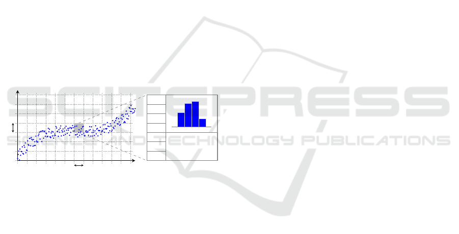
The model tries to capture the distribution of a given

stream (roughly its “shape”). In order to achieve

this it discretises the streams into same size buckets,

computing the probabilities to traverse those buckets.

Only the previous bucket is used as a state for the

probability vector, as such the model can be consid-

ered a ﬁrst order Markov chain. At the same time,

the buckets themselves could store some local statis-

tics about the distribution of the points falling within

them to better represent the real streams. A visual

representation of the model is presented in Figure 1.

∆x

∆y

Figure 1: Structure proposed to represent stream informa-

tion. A grid is overlayed over the streams, in order to build a

matrix like structure where each slot contains a probability

vector, a histogram of values, and other relevant statistical

values (e.g. the mean and standard deviation of the values

inside the slot).

2.2 Generative Adversarial Network

(GAN)

GANs (Goodfellow et al., 2014) are a new architec-

ture of networks which aims at modelling the distri-

bution of some dataset based on ideas borrowed from

game theory (Salimans et al., 2016).

GANs work by considering two adversarial net-

works, called discriminator and generator. The for-

mer is trained to distinguish “fake” samples, those

generated by the generator, from those of real data.

Meanwhile, the latter is trained to produce samples

capable of fooling the discriminator, making it believe

its generated samples are real. This can be understood

as a minimax game, where the discriminator trains to

maximize its probability of assigning correct labels

to both real and generated samples, while simultane-

ously the generator tries to minimize the probability

of the discriminator correctly doing so. Ultimately,

one is hopefully left with a discriminator which shows

an accuracy of around 50%, meaning that it mostly

guesses the origin of the data presented to it.

In the original paper (Goodfellow et al., 2014) the

authors suggested the usage of Multilayer Perceptrons

(MLPs) for both the discriminator and generator. Nat-

urally the research community was keen to experi-

ment with other architectures, conducing in (Radford

et al., 2015) to the proposal of using Convolutional

Neural Networks (CNNs) instead of the initially sug-

gested MLPs. This new architecture, coined Deep

Convolutional GANs (DCGANs) by its authors, was

more stable than the previous to train, while still very

capable of learning generative models.

The generative capabilities of GANs have already

been extensively studied for image data, for instance

in all the previously mentioned papers (Goodfellow

et al., 2014,Radford et al., 2015,Salimans et al., 2016)

dealing with (DC)GANs.

In fact, generating images has been the standard

way of evaluating the quality of GANs’ architectures,

since it is easy to visually determine whether a gener-

ator is behaving properly or not. Moreover, it is com-

mon to employ GANs when one wants networks to

learn features which can later be used in other tasks

(employing transfer learning for instance), which usu-

ally involve image data. All the previously mentioned

papers show that GANs are in fact capable of learning

these features and generating more or less reasonable

images, with their quality of doing this evolving as

the techniques used also become more reﬁned.

Despite this, GANs (and particularly DCGANs)

have not been as widely employed when dealing with

non-image data. Most likely stems from the fact that

deep learning is typically associated with images and

not so much with other data.

Convolutional networks in GANs behave as they

usually do in other architectures, taking advantage of

the locality which is implicit in image data (i.e. re-

gions which are close together have strong meaning,

while relations between regions far apart do not have

as much). Yet, these intrinsic properties may be found

in other scenarios as well, for instance in sequential

data such as time series.

It has already been shown in a previous paper (An-

tunes et al., 2017, Jesus et al., 2018) that the distri-

bution of a given stream of sensorial data could be

modelled by ﬁrst order Markov chains. However, this

model was ﬁrst developed with stream similarity in

IoTBDS 2019 - 4th International Conference on Internet of Things, Big Data and Security

178

mind, not stream generation, but it was shown to be

quite capable at the latter task as well.

It thus becomes interesting to evaluate whether a

Markov chains-free model can be built and trained,

resorting to DCGANs, which is capable of competi-

tively learning the distribution of data streams.

3 DATA PREPROCESSING

3.1 Dataset Description

In this paper we used a dataset collected at Intel

Berkeley Research lab

. It comprises records of tem-

perature, humidity, light and voltage measured once

every 31 seconds by 54 sensors for the duration of

approximately one month (March, 2004).

Due to the amount of time it takes to train the mod-

els, we have focused primarily only on the tempera-

ture measures of the dataset.

We have separated the stream of values produced

by each sensor by day, which resulted in a total of

1674 streams. It should be noted that this is “raw”

data, with minimal to no preprocessing involved. As

such, the number of streams selected for training was

signiﬁcantly smaller (more details regarding this issue

can be found in section 3).

A plot illustrating these streams is presented

in Figure 2.

The presence of outliers becomes clear by look-

ing at the plots. To further support this point, notice

that the maximum reading measured by a sensor is

294.3

◦

C, and the minimum of −38.4

◦

C. It is obvi-

ously highly doubtful that the sensors have indeed ex-

perienced such extreme temperatures inside an ofﬁce.

3.2 Dataset Preprocessing

The ﬁrst step into transforming this data into a more

workable format was to separate the streams by day

and by sensor. This resulted in 1674 different streams.

Afterwards, given that we intend to train different

models (involving Markov chains and GANs) with

this dataset (which will have a ﬁxed number of in-

puts), we processed the streams so that all have the

same number of data points.

Since each sensor recorded temperatures around

once every 30 seconds (although many missing points

exist), it was decided that each stream would be com-

posed of 24×60 = 1440 data points, i.e. one point per

minute.

http://db.csail.mit.edu/labdata/labdata.html

In order to do this the time of each day

was discretized into regions with boundaries

{0, 60, 120, . . . , 24 × 60 × 60}. Then, points of a

stream falling within consecutive boundaries were

reduced to a single point by computing their median.

To slots without any points, the label nan was

assigned. We do not interpolate these values at this

stage since we use the amount of missing values

as an indicator of the quality of the stream, which

eventually helps deciding whether the sample should

be dropped or not.

Figure 2 plots the streams obtained up to this point

in preprocessing.

3.3 Outliers and Missing Values

Having now the streams laid in a structure which was

easier to work with, we turned our attention to iden-

tifying and removing outliers in the data (which are

quite noticeable just by looking at the plots) and to

handle missing values (the library used to train the

networks does not work with “not a numbers” —

nans).

Outlier detection was based on the modiﬁed Z-

score proposed by Iglewicz and Hoaglin in (Iglewicz

and Hoaglin, 1993). This is essentially a more ro-

bust version of Z-score which replaces the mean by

the median and the standard deviation by the median

absolute deviation (MAD). It is deﬁned as

0.6745(x

− ˜x)

MAD

where MAD = median(

− ˜x

) and ˜x denotes the me-

dian of x.

The authors suggest that modiﬁed Z-scores with

an absolute value greater than 3.5 should be consid-

ered (potential) outliers. This was the test that we em-

ployed. Outliers identiﬁed with the previously men-

tioned technique are labelled as nan (same as had

been done for missing values).

At this point, we ﬁlter out streams which have too

many points labelled nan. The threshold used for this

is to remove streams which do not have a count of at

least 70% of the points they are expected to have (at

one per minute this is 0.7 × 24 × 60 = 1008).

After this step we are left with 700 streams (ver-

sus the initial 1674, which further suggest the heavy

presence of outliers/missing values).

Finally, in order to resolve the missing values, the

streams were linearly interpolated, so that the points

labelled nan are replaced with hopefully reasonable

ones.

The resulting streams after preprocessing are il-

lustrated in ﬁgure 3.

Stream Generation: Markov Chains vs GANs

179

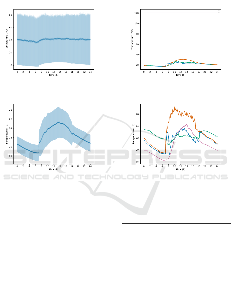
Figure 2: Raw temperature data used. To the left, in bold the mean (µ) of temperature readings at each instant of the day.

In light shade the region captured by the standard deviation (σ) of those readings, i.e. [µ − σ, µ + σ]. To the right, randomly

selected samples of the set of streams.

Figure 3: Temperature data used after preprocessing. The meaning of the ﬁgures is the same as those in ﬁgure 2.

4 IMPLEMENTATION

This section will elaborate on both approaches

(Markov chains and GANs) to stream generation, ex-

plaining their implementations.

We will start by brieﬂy discussing the implemen-

tation using Markov chains, referring the interested

reader to the main paper presenting this approach.

Afterwards, we will elaborate on the implementation

around GANs (with greater focus due to its novelty).

This section is more extensive since we have not pre-

sented it before.

4.1 Markov Chains

As previously stated, this model has already been de-

tailed previously in (Antunes et al., 2017, Jesus et al.,

2018). In order to keep this paper self-contained,

we will provide a small brieﬁng of this technique

here. Essentially this method works by laying a grid

over a stream/set of streams and then, from this train-

ing sample, extrapolate the probabilities of being in

slot (x

i+1

, y

) given that the stream was previously in

, y

). The algorithm used to generate a stream from

a previously trained model is depicted in Algorithm 1.

Algorithm 1: Stream Generation.

1: function GENERATESTREAM(model, yinit)

2: bin ← (0, yinit)

3: genstream ← {Gener atePoint(model, bin)}

4: for i ← 1, #ColumnsO f (model) − 1 do

5: bin ← GenerateNextBin(model, bin)

6: genstream ←

genstream

{GeneratePoint(model, bin)}

7: end for

8: return genstream

9: end function

The function GeneratePoint uses the histogram

of a model’s bin to generate a point in accordance with

IoTBDS 2019 - 4th International Conference on Internet of Things, Big Data and Security

180

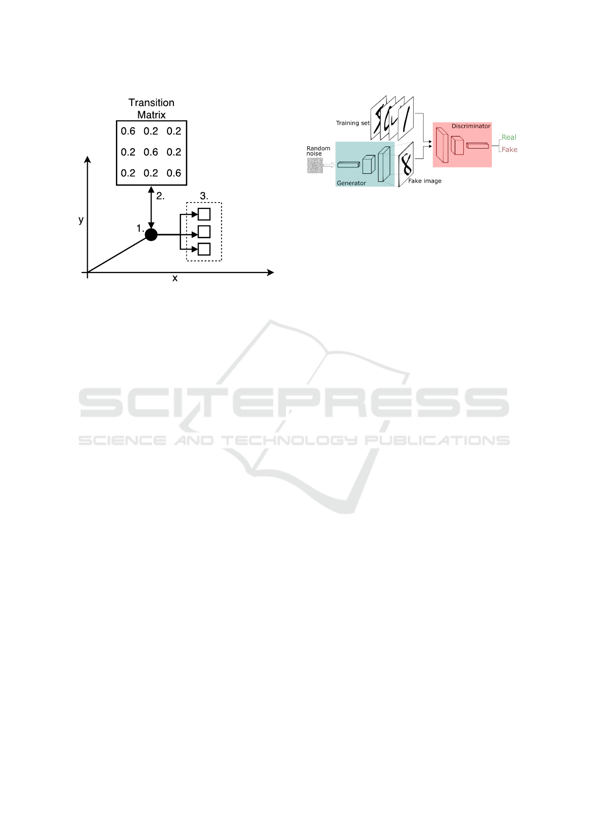
Figure 4: Generation process. 1. at each bucket, generate

a random value that represents the transition probability;

2. use the transition matrix to identify the next bucket; 3. at

the destination bucket, generate a new value (based on its

histogram).

its distribution. The function GenerateNextBin uses

the probability vector of a bin to determine where the

generated stream will ﬂow through. In Figure 1 is

depicted a visual representation of the model being

used for stream generation. As a ﬁnal note, the ac-

tual implementation of these methods and associated

data structures was carried out in Python3, resorting

mainly to the standard libraries, numpy and scipy.

4.2 GANs

Some notions about GANs and DCGANs were al-

ready provided in Section 2. Here we will be more

speciﬁc regarding the architecture of the networks

used as well as how its training was conducted.

4.2.1 Generative Adversarial Networks (GANs)

GANs, the super type of DCGANs, work by pitting

two networks, a discriminator and a generator, against

one another. The ﬁrst, the discriminator, will try to

classify input samples presented to it as being real or

synthesized ones. Meanwhile, the generator will try

to learn how to generate samples which trick the dis-

criminator into labelling fake data as valid. The over-

all concept is illustrated in ﬁgure 5.

Typically, for training, one network is deployed

for the discriminator, and two (stacked) for the gen-

erator. The latter is composed of the actual generator

per se stacked with the discriminator. As will be seen,

while training the generator only its actual generative

network is modiﬁed. Training the discriminator is car-

Figure 5: How a GAN works at an high level. Source:

https://medium.freecodecamp.org/an-intuitive-introduction-

to-generative-adversarial-networks-gans-7a2264a81394

ried as usual, providing it with real samples alongside

“valid” labels and generated samples with “fake” la-

bels.

Meanwhile, training the generator involves more

actions underneath. In essence the generator is pro-

vided with noise (typically from a normal distribu-

tion) alongside labels stating “valid” samples. Notice

that despite the generator also comprising the discrim-

inator network as seen above, the latter is locked for

training at this stage. As a result, the weights that can

change and adapt are only those of the actual gener-

ator part of the network, which will as a result try to

learn how to produce samples that fool the discrimi-

nator succeeding it.

It becomes apparent at this stage that the generator

will only be as good as the discriminator is. The better

the latter is, the more the former will feel pressured

into producing realistic samples.

4.2.2 Deep Convolutional GANs (DCGANs)

Having in mind the overall idea behind GANs, it is

time for discussing actual architectures for the dis-

criminator and generator networks.

The initial paper presenting GANs (Goodfel-

low et al., 2014) suggested Multilayer Perceptrons

(MLPs) for both discriminator and generator. Yet,

more recent research (Radford et al., 2015, Salimans

et al., 2016) has found success with Convolutional

Neural Networks for both networks. This is the ap-

proach also followed in the present work. As for the

generator network, its architecture is inspired on the

original DCGAN paper (Radford et al., 2015) and is

presented in ﬁgure 6.

In the original paper the authors had started with a

convolutional layer of depth 1024, yet here only 512

is used. This is also the approach followed by (Sali-

mans et al., 2016), the paper on improved techniques

for training GANs by (some of) their original authors.

The network receives 100 latent values (noise) and

from these it is expected to produce, at its last layer, a

32 × 32 image with three channels (RGB).

Stream Generation: Markov Chains vs GANs

181

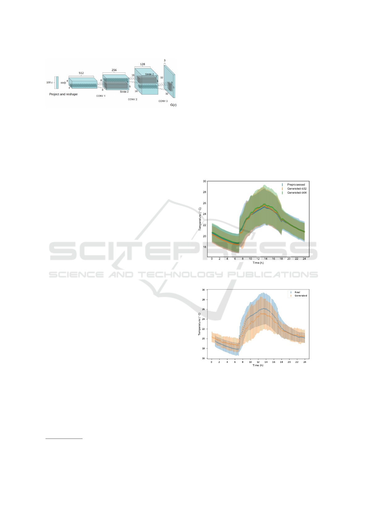
Figure 6: Concept design for the DCGAN’s genera-

tor. Source: Adapted from the original paper on DC-

GANs (Radford et al., 2015)

In the present case we are not interested in gener-

ating images and as a result we had to adapt the archi-

tecture in order to ﬁt our requirements. The overall

design is kept the same, but the actual dimensions of

the layers comprising the generator are

(1 80 ,5 12 ) -> (3 60 ,2 56 ) -> (7 20 ,1 28 ) -> ( 1440 ,1)

Notice that the ﬁrst dimension keeps on increasing

due to upsampling, a procedure where the units on a

layer are replicated a certain number of times (in this

case 2) along certain directions. Interestingly, usually

in CNNs one does the opposite and employs down-

sampling in order to reduce the number of units.

In all but the last layer a kernel of size 5 was used

as well as batch normalization and ReLU as the acti-

vation function. The last layer uses Tanh for activa-

tion, which is in accordance with suggestions found

in the previously mentioned papers.

Regarding the discriminator network, it is a some-

what more common CNN. It is comprised of 4 con-

volutional layers and 1 dense layer. The convolu-

tional layers are progressively more deep, starting at

32 and multiplied by two up to 256. For these lay-

ers LeakyReLU is used as activation function and

dropout as regularization mechanism. The dense

layer has a single node and uses the sigmoid function

for activation.

Although the papers mentioned previously do not

discuss in depth architectures for the discriminator

network, the considerations they make about it (e.g.

the usage of batch normalization) were taken into ac-

count.

The Keras library

was used for the prototyping of

the networks. The DCGAN implementation at https://

github.com/eriklindernoren/Keras-GAN was used as

starting point for development. Modiﬁcations to make

it work with stream data (1D) as opposed to im-

age data (2D) were required, as well as adjustments

to training parameters as will be seen in Section 5,

mainly since the default ones in the original imple-

mentation did not allow the networks to converge fast

enough.

https://keras.io/

5 RESULTS AND EVALUATION

Due to time constraints it was impossible to evaluate

both models with proper detail, and compare them

with other generators. Nevertheless, in this section

we present and discuss the initial results. Both mod-

els were trained on the previously mentioned dataset

(subsection 3.1). It is important to notice that we pro-

vide more details to the GAN model since it is being

published for the ﬁrst time.

Two batch sizes were considered for training the

GANs: 32 and 64. In Figure 7 it is depicted the result

of the model after training. Multiple generations pro-

duced by the the model were overlapped on top the

original data. The same was done to the Makov based

model (see Figure 8)

Figure 7: Multiple generated stream (GANs) overlapped on

top the original data.

Figure 8: Multiple generated stream (Markov) overlapped

on top the original data.

It is possible to verify that both models appear to

capture the overall “shape” that characterizes this par-

ticular phenomenon. It is also important to mention

that there are no visible difference when considering

the used batch sizes. Nevertheless, the resolution of

the model appear to be better when GANs are used.

This is to be expected, the deep structure that an ar-

tiﬁcial neural network allows it to learn a model with

IoTBDS 2019 - 4th International Conference on Internet of Things, Big Data and Security

182

higher resolution (and accuracy). Keep in mind that

the Markov model was designed with stream similar-

ity in mind. Taking this into account, and the simplic-

ity of the model (which implies faster training times)

makes the Markov model more than sufﬁcient for sev-

eral real world scenarios.

Table 1 presents a comparison between both mod-

els. In short, the model based on GANs provides

more ﬂexibility and resolution when considering only

stream generation. Nevertheless, keep in mind that in

order to achieve the desired resolution may be nec-

essary to tune the hyper-parameters until sufﬁcient

accuracy is achieved. On the other hand, the model

based on Markov chain was designed for stream sim-

ilarity, only provides moderate resolution. Although

the size of the bucket can be adjusted, the model only

used the previous state in order to compute the next

bucket, in this regards the model is shallow. The lack

of ﬂexibility is compensated with a simpler training

method and faster execution.

Table 1: Comparison between Markov and GANs model for

stream generation.

Features/Model Markov GANs

Training time Fast Slow

Model size Small Large

Generation time Fast Fast

Resolution (accuracy) Moderate High

Stream Similarity Capable NA

Hyper-parameters Limited Flexible

6 CONCLUSION

The number of sensing devices is increasing at a

steady step. Each one of them generates massive

amounts of information. This lead to a new genera-

tion of IoT and M2M platforms that capture the pre-

viously mentioned information and provide context-

aware services. Currently these platforms use ad-

vanced machine learning algorithms to improve and

optimize several processes. Having the ability to test

them for a long time in a controlled environment is

extremely important. The ability to generate streams

resembling a given set of learning ones can be useful

in this situation. Stream generators can be used ver-

ify and improve the repeatability and validity of IoT/

M2M and context-aware platforms.

Both models discussed in this publication can be

used for this task. Nevertheless, there are several dif-

ferences between them. GAN based models provide

better resolution and ﬂexibility at the cost if longer

training times and ﬁne-tuning. On the other hand,

Markov models provide moderate resolution, can be

used to estimate similarity between streams and are

fast to train.

Due to time constrains the evaluation and com-

parison between the models lacked sufﬁcient detail.

We intend to address this issue in a future publication,

with a larger dataset for validation. It is important to

notice that generator based on the ﬁrst order Markov

chain is still under research. Several improvements

will be proposed in the future, such as methods to es-

timate the bucket size autonomously.

ACKNOWLEDGEMENTS

This work is funded by FCT/MEC through national

funds and when applicable co-funded by FEDER

– PT2020 partnership agreement under the project

UID/EEA/50008/2019.

REFERENCES

Antunes, M., Jesus, R. J., Gomes, D., and Aguiar, R. L.

(2017). Improve iot/m2m data organization based on

stream patterns. In 2017 IEEE 5th International Con-

ference on Future Internet of Things and Cloud (Fi-

Cloud), pages 105–111.

Chen, K.-C. and Lien, S.-Y. (2014). Machine-to-machine

communications: Technologies and challenges. Ad

Hoc Networks, 18:3–23.

Datta, S. K., Bonnet, C., Costa, R. P. F. D., and Härri, J.

(2016). Datatweet: An architecture enabling data-

centric iot services. In 2016 IEEE Region 10 Sym-

posium (TENSYMP), pages 343–348.

Fantacci, R., Pecorella, T., Viti, R., and Carlini, C. (2014).

Short paper: Overcoming iot fragmentation through

standard gateway architecture. In 2014 IEEE World

Forum on Internet of Things (WF-IoT), pages 181–

182.

Goodfellow, I., Pouget-Abadie, J., Mirza, M., Xu, B.,

Warde-Farley, D., Ozair, S., Courville, A., and Ben-

gio, Y. (2014). Generative adversarial nets. In Ghahra-

mani, Z., Welling, M., Cortes, C., Lawrence, N. D.,

and Weinberger, K. Q., editors, Advances in Neu-

ral Information Processing Systems 27, pages 2672–

2680. Curran Associates, Inc.

Iglewicz, B. and Hoaglin, D. (1993). How to Detect and

Handle Outliers. ASQC basic references in quality

control. ASQC Quality Press.

Jesus, R., Antunes, M., Gomes, D., and Aguiar, R. L.

(2018). Modelling patterns in continuous streams of

data. Open Journal of Big Data (OJBD), 4(1):1–13.

Perera, C., Zaslavsky, A., Christen, P., and Georgakopoulos,

D. (2014). Context aware computing for the internet

of things: A survey. IEEE Communications Surveys

Tutorials, 16(1):414–454.

Stream Generation: Markov Chains vs GANs

183

Radford, A., Metz, L., and Chintala, S. (2015). Un-

supervised representation learning with deep con-

volutional generative adversarial networks. CoRR,

abs/1511.06434.

Robert, J., Kubler, S., Traon, Y. L., and Främling, K. (2016).

O-mi/o-df standards as interoperability enablers for

industrial internet: A performance analysis. In IECON

2016 - 42nd Annual Conference of the IEEE Industrial

Electronics Society, pages 4908–4915.

Salimans, T., Goodfellow, I., Zaremba, W., Cheung, V.,

Radford, A., Chen, X., and Chen, X. (2016). Im-

proved techniques for training gans. In Lee, D. D.,

Sugiyama, M., Luxburg, U. V., Guyon, I., and Garnett,

R., editors, Advances in Neural Information Process-

ing Systems 29, pages 2234–2242. Curran Associates,

Inc.

Wortmann, F., Flüchter, K., et al. (2015). Internet of

things. Business & Information Systems Engineering,

57(3):221–224.

IoTBDS 2019 - 4th International Conference on Internet of Things, Big Data and Security

184