Smart Parking Zones using Dual Mode Routed Bluetooth Fogged Meshes

Paul Seymer

, Duminda Wijesekera

and Cing-Dao Kan

Radio and RADAR Engineering Laboratory, George Mason University, Fairfax, VA 22030, U.S.A.

Center for Collision Safety and Analysis, George Mason University, Fairfax, VA 22030, U.S.A.

Keywords:

Smart Parking, Bluetooth, Mesh Networking.

Abstract:

Contemporary parking solutions are often limited by the need for complex sensor infrastructures to perform

space occupancy detection, and costly to maintain ingress and egress parking systems. For outdoor lots, net-

work infrastructure and computational requirements often limit the availability of innovative technology. We

propose the use of Bluetooth Low Energy (BLE) beacon technology and low power sensor nodes, coupled

with sensible placement of computational support and data storage near to the sensor network (a Fog comput-

ing paradigm) to provide a seamless parking solution capable of providing parking maintainers with accurate

determinations of where vehicles are parked within the lot. Our solution is easy to install, easy to maintain,

and does require signiﬁcant alterations to the existing parking structures.

1 INTRODUCTION

Modern smart parking solutions have many prob-

lems. First, many suffer from the need to install per-

space sensors to provide accurate occupancy detec-

tion. Others require too much user interaction, such

as using smartphone apps to scan space identiﬁers.

Other solutions use isolated ingress and egress pay-

ment interaction points, entailing costly automation.

While the original intent of technology deployments

to parking lots was to make management cost effec-

tive and usable, contemporary commercial solutions

continue to use old paradigms and fail to achieve

seamless, low cost, low resource intensive but service

rich parking management solutions.

Parking lots, particularly outdoors often reside

outside wireless (or even wired) network boundaries.

Additionally, these spaces have minimal power to

support lighting and other basic infrastructure. Sug-

gesting a complicated technology stack for deploy-

ment to these lots will replace one problem with an-

other and become cost prohibitive. Shifting to cloud

computing technology offer the ability to take advan-

tage of high computational ability without the over-

head and expense of maintaining it, nor paying for

its use when idle. One major drawback of this tech-

nology is the dependence on a reliable, and often

large, network connection, a rarity in parking lots.

Fog computing, counters such dependencies by shift-

ing computation and storage closer to the parts of a

network that need them. In the case of sensor net-

works, like the ones that are deployed to smart park-

ing lots for occupancy detection, Fog computing sug-

gests that storage and computational capability be lo-

cated as close to the network’s sensor capability as

possible. This is a challenge, as the devices that per-

form sensor activities are often low power, and as a re-

sult have extremely limited storage and computational

capability. What is needed is a low cost, low power

solution with minimal user interaction to function.

Doing so requires eliminating traditional ingress and

egress payment and tracking support and replacing it

with something completely seamless that does not in-

terfere with vehicle ingress or egress or to/from the

lot. Occupancy detection must not have a one-sensor-

per-space requirement. Deployment of the solution

should not require signiﬁcant alteration of the exist-

ing lot. We suggests using low cost, low power, Blue-

tooth Low Energy (BLE) sensors and BLE beacon

technology to create a fully automated and seamless

parking experience. In this paper, we improve upon

our prior work (Seymer et al., 2019) in several ways:

Improved localization, simpliﬁed machine learning

model (smaller feature vector), signiﬁcantly lower

mesh network overhead during operation, and adapta-

tion of Fog/Cloud concepts to provide on-demand and

off-network computation (simplifying on-lot compu-

tation demand). We compare this to a solution that

use an Edge Computing object recognition camera as

a BLE vehicle attestation to our solution.

Seymer, P., Wijesekera, D. and Kan, C.

Smart Parking Zones using Dual Mode Routed Bluetooth Fogged Meshes.

DOI: 10.5220/0007734802110222

In Proceedings of the 5th International Conference on Vehicle Technology and Intelligent Transport Systems (VEHITS 2019), pages 211-222

ISBN: 978-989-758-374-2

211

2 PROPOSED SOLUTION

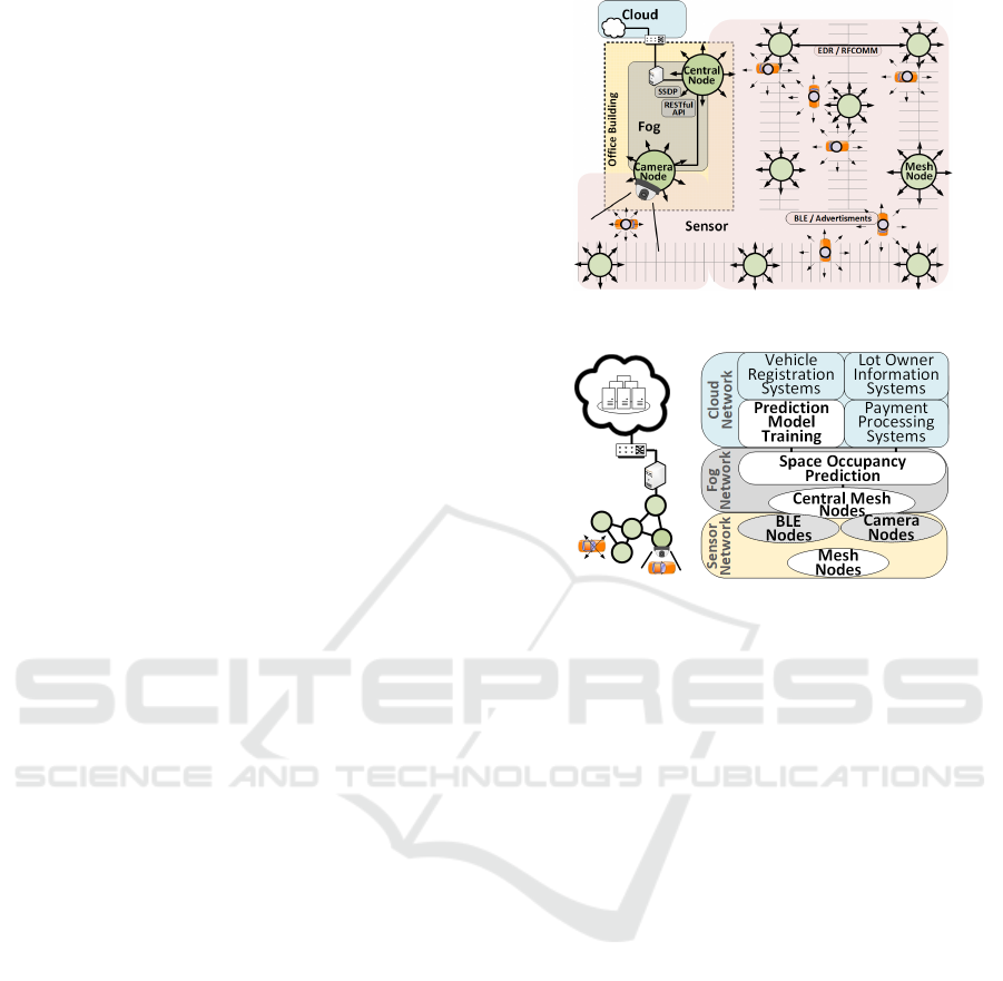
An overview of our solution is shown in Figure 1

where the target parking lot is equipped with Blue-

tooth sensor nodes that measure radio strength from

vehicles equipped with BLE beacons. These sensor

nodes form an authenticated mesh network, based off

of real-time radio signal strength between them to al-

low the network to self-form and adapt to changing

conditions like interference or node failure. When

vehicles enter the lot and park, the sensor network

records Received Signal Strength Indicator (RSSI)

values and relays these values over Bluetooth Clas-

sic (RFCOMM connections) to a central node. This

central node assembles the sensor data together and

performs a space prediction activity using a Random

Forest machine learning model, trained against a ra-

dio map created at installation time. This model was

trained ofﬂine to simulate an activity we see as occur-

ring in a real-life deployment in the cloud, however

the size of our parking lot and the low-density of sen-

sor nodes is such that training this model could have

been performed on a host within the fog network. Our

solution takes advantage of edge computing and fog

computing by conﬁguring the sensor nodes with sam-

ple rates and other data pre-processing steps aimed at

reducing network demand, performing execution of

the space prediction activity on a power unrestricted

fog network located within a nearby ofﬁce building,

and ofﬂoading lot-agnostic or global activities such as

trending and payment processing to the cloud. Here,

all computations needed to make a space determina-

tion is located on the fog network, sparing the connec-

tion to the cloud from this additional demand. Exter-

nal services that can beneﬁt from this data can interact

directly with the cloud, sparing the fog and sensor net-

works from supporting those processes. This arrange-

ment is shown in Figure 2. In addition, our system

detects vehicles that enter and exit the lot, and authen-

ticates them. We do so with two solutions, one based

purely on Bluetooth radio, and another that combines

the radio with an object recognizing camera deployed

to an ingress point at the parking lot. We experimen-

tally contrasted both solutions.

2.1 Parking Space Occupancy Detection

Our space occupancy prediction model is an evolu-

tion of prior work (Seymer et al., 2019), where we

used RSSI values from Bluetooth beacons, measured

at multiple locations within a parking lot to train a

Random Forest machine learning classiﬁer. This sec-

tion outlines signiﬁcant changes and improvements to

that work, and new features provided by our current

Figure 1: Solution Overview.

Figure 2: Cloud, Fog, and Sensor Network Model.

system.

2.1.1 Zone based Occupancy Detection

Preliminary experiments were performed with a per-

space occupancy detection goal. Results were accu-

rate above 90% for our training set for all spaces in

the lot, with less accurate spaces along the south and

south east corners of the lot (marked as orange circles

in Figure 3). Suspecting that this was due to signal

interference in the 2.4GHz range from the surround-

ing residential area, we considered zoned-based oc-

cupancy detection instead of individual spaces as a

mitigation technique, as parking lot owners will most

likely not want a pricing model that differs between

spaces that border one another, except for regions

such as near a building entrance, or on a level of a

parking garage. Consequently, we use zones consist-

ing of contiguous spaces as shown in Figure 3.

2.1.2 Sensor Node Placement

To avoid deploying structures that impede trafﬁc ﬂow

or compromise existing spaces, we used existing lamp

posts to mount nodes at heights of 8 feet or more. Two

sensor nodes are located within the nearby building

that belong to both the BLE sensor network and the

fog network, to act as a network bridge to allow for

sensor data to be used off-network for payment, etc.

(see Figure 3).

VEHITS 2019 - 5th International Conference on Vehicle Technology and Intelligent Transport Systems

212

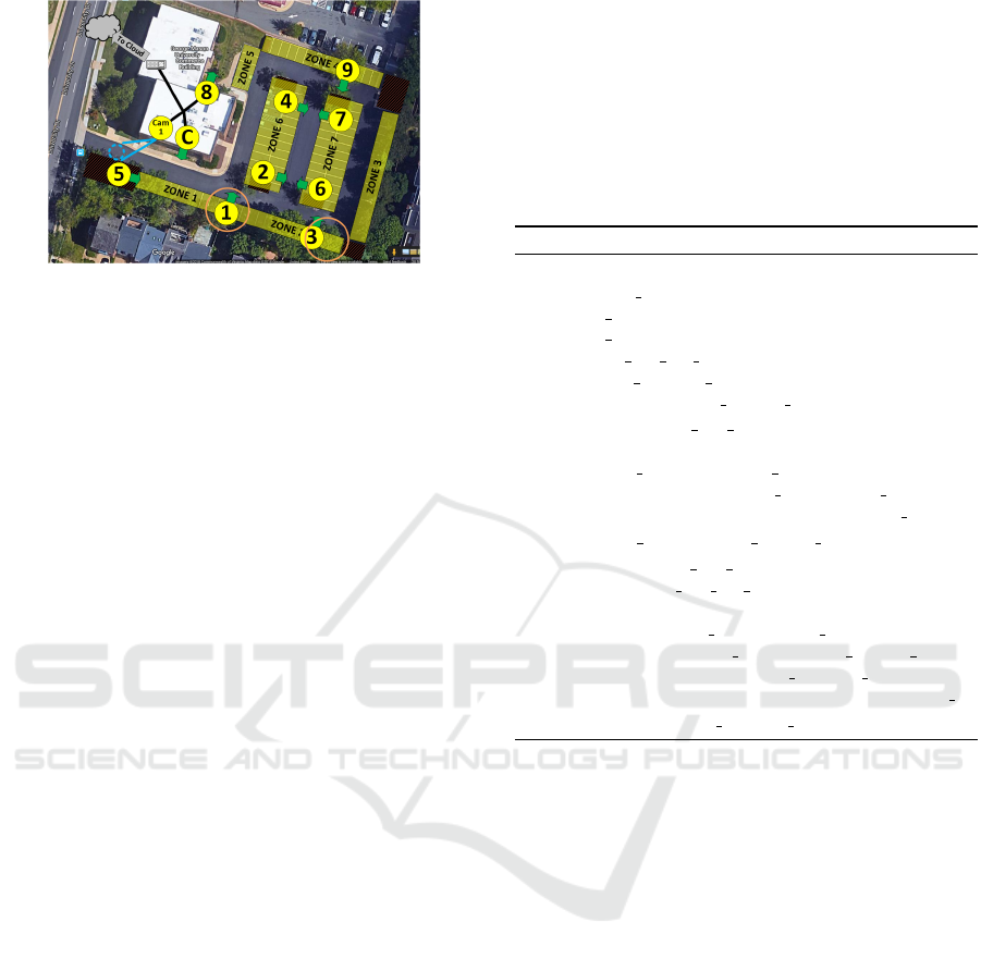
Figure 3: Parking Space Zone Map.

Preliminary experiments in prior work with a 7

node network resulting in mis-classiﬁcations primar-

ily involving spaces in zones 2 and 3 in both the train-

ing set and the in-vehicle testing. Additionally, the

formed mesh routed all trafﬁc through node 1, cre-

ating a a single point of failure and a potential bot-

tleneck, should the network become saturated. As a

mitigation, we deployed two additional sensor nodes

to address inaccurate predictions for nearby spaces in

zones 2, 3 and 4, and a third node on the other side of

the building (near node 4, not shown in the ﬁgure) to

allow for multiple mesh paths to be formed with the

nodes inside the building.

2.1.3 Radio Fingerprint Feature Selection

Our ﬁrst features included many statistical measures

of RSSI values and their changes over time. After

consequent analysis, we removed features with min-

imal positive value to the model. An example is the

median count of RSSI beacons seen over discrete time

intervals. In practice, this metric varied greatly once

a beacon was placed inside a vehicle, creating higher

errors in prediction. Such issues are addressed in

Section 3.1.3. Temporary physical obstructions cause

signal attenuation or in some cases prevent a beacon

measurement entirely. To mitigate this effect, we used

the highest observed RSSI value per node per space,

as this gave the best result. Our experiments described

in Section 3 support this choice.

2.1.4 Bluetooth-only Vehicle Identiﬁcation and

Tracking

Due to the range of Bluetooth, each space is observ-

able from several sensors in our network. When a

vehicle enters the lot and parks, its unique beacon

broadcast will be detected as part of the localization

process. If that beacon has not been seen for a period

of time, we assume that the vehicle has exited the lot.

Our process for vehicle detection and identiﬁcation

is shown in Algorithm 1. Initialization is run when

the network is started, shown in lines 1-7. This algo-

rithm maintains a data structure of observed beacons

(lines 8-12), launches a thread (line 7) to observe this

data structure (line 16) and determine when a vehicle

has exited the lot (line 18). If an exited vehicle is de-

tected, a notiﬁcation is sent (line 19) so that external

functions could be run to initiate payment and other

business functions based on lot occupancy.

Algorithm 1: BLE Only Vehicle Identiﬁcation Procedures.

1: procedure initialize()

2: parked records ← {}  init history data structure

3: veh entered ← {}  init enter records

4: veh exited ← {}  init exit records

5: detect veh kill ﬂag = False

6: beacon measure intvl = 5min

7: start thread detect vehicle exit()

8: procedure detect veh enter(each received beacon b)

 called for each beacon central receives

9: if b.veh id not in parked records then

10: create entry for b.veh id in parked records

11: notify mgr new vehicle parked (b.veh id)

12: parked records[b.veh id].last seen ← b.time

13: procedure detect veh exit()

14: while detect veh kill ﬂag = False do

15: n ← time.now()

16: for each veh rec ∈ parked records do

17: r ← parked records[b.veh id].last seen

18: if (n − r) > beacon measure intvl then

19: notify mgr new vehicle exited (b.veh id)

20: sleep (beacon measure intvl)

One potential gap in our solution is the assump-

tion that a beacon found within a lot is indeed inside

a vehicle, and that all vehicle entering the lot have an

active beacon. While our smart parking solution will

only be deployed to lots that have 100% participation

by all vehicles, we are sensitive to the potential for

a malicious vehicle operator entering the lot without

powering their beacon. To our solution, this would

not appear as a space occupying vehicle at all, but we

explore a solution to this in the next section.

2.1.5 Camera-based Vehicle Detection and BLE

Beacon Attestation

To remedy the potential for vehicles to evade detec-

tion by disabling their beacons, we explore the use

of a low cost, low power object recognition camera

located at the entrance/exit points of the lot. We

selected the Jevois-A33 Smart Camera (JeVois Inc,

2018), an all-in-one camera and CPU with a USB in-

terface, chosen primarily due to its low price point

(under $60 USD), and the ability to recognize objects

out-of-the-box with little conﬁguration. We conﬁg-

ured the camera to recognize vehicles using the Jevois

Smart Parking Zones using Dual Mode Routed Bluetooth Fogged Meshes

213

Darknet YOLO module (Itti, 2018) which employs

YOLOv3 (Redmon and Farhadi, 2018), a neural net-

work that quickly detects objects based on a single

pass across an image obtained from the camera. We

connected the camera using USB to one of our mesh

nodes and we use the camera’s USB interface and

sent serial messages from its classiﬁer to its built-in

logging module. The node connected to the camera

was also equipped with a BLE receiver and observe

nearby beacons and discover if the vehicle viewed by

the camera has a valid active beacon - assuring that the

speciﬁc beacon observed does indeed correspond to a

car. While a simple solution, we view this as a prelim-

inary step for augmenting our BLE-only solution with

additional low cost low development attestations. We

conducted feasibility experiments for this implemen-

tation in Section 3.3, and contrast this solution with

the BLE only solution in Section 2.1.4. We outline

how this arrangement functions in Algorithm 2. Algo-

rithm initialization occurs (lines 1-6), creating a data

structure, populated by two watcher threads that ob-

serve and record BLE beacons and camera-based ob-

ject detections. Additionally, two thresholds are set

specifying the RSSI value required by a beacon to in-

dicate it is near to the camera node (line 5), and the

maximum time difference between a camera recogni-

tion event and a matching BLE beacon (line 6). When

a vehicle passes near the camera, it is recognized by

the camera’s object recognition system and logs a de-

tection event through the serial connection to its node.

Additionally, the vehicle’s beacon is observed by the

BLE receiver on the node. As BLE beacon detection

and camera-based object recognition are independent

processes, a step is required (lines 11-14) to match

them based on similar time-stamps deﬁned by our

threshold (line 6). Section 3 experimentally shows

that camera recognition takes a few extra seconds to

process when compared to the BLE detection. This

occurs because the radio broadcast of slow moving

cars reaches the camera node’s BLE sensor before the

vehicle comes into the camera’s view. Once the match

occurs, this attestation event is passed back to the cen-

tral node for use (line 16) or an error is sent if a bea-

con or camera event are missing (line 18). Lastly, our

experiments show that the camera does not function

at night when there is insufﬁcient light to recognize

objects correctly, so this algorithm is only run during

daylight hours (lines 7-8).

2.2 Fogged BLE Sensor Meshnet

Our solution is composed of software-identical nodes,

assigned and conﬁgured to a speciﬁc roles: mesh

network, sensor, in-vehicle, or camera. Any node

Algorithm 2 : Hybrid BLE/Camera Vehicle Identiﬁcation

Procedures.

1: procedure initialize

2: Initialize datastructure d

3: Start thread to record BLE beacons

4: Start thread to record events from camera

5: bt ← rssi threshold (set to -70 dBm)

6: td ← event time delay (set to 5 seconds)

7: if is nighttime then

8: Exit, as camera does not function at night

9: procedure attest veh thread(datastructure d)

10: if d has new event e then

11: if e is a new Beacon event b then

12: Find matching Camera event c

13: if e is a new Camera event c then

14: Find matching Beacon event b

15: if both c and b do not exist then

16: Send error (-,b or c,-) to central node

17: else

18: Send attestation (c,b) to central node

can perform any role provided it is equipped with

the necessary hardware, allowing deployment activ-

ities to place sensor nodes where they are needed

for detection, and if needed, turn them into network

nodes at a later time. The mesh network is formed

over Bluetooth Classic (EDR Mode), partially insu-

lating the BLE-based occupancy prediction function-

ality from radio interference. Nodes that must com-

municate inside buildings and to upper network lay-

ers (i.e. Cloud) do so over the building’s existing

wired network to reduce the in-building mesh net-

work density required to compensate for signal atten-

uation from walls and ﬂoors. As one of the nodes

on this fog network was the central node, this wired

network formed the basis for the internal boundary of

our fog network. Once we determined which parame-

ters we would use for our space prediction algorithm,

we conﬁgured the sensor nodes to sample data and

perform initial processing to reduce network trafﬁc

and computational requirements for the central node.

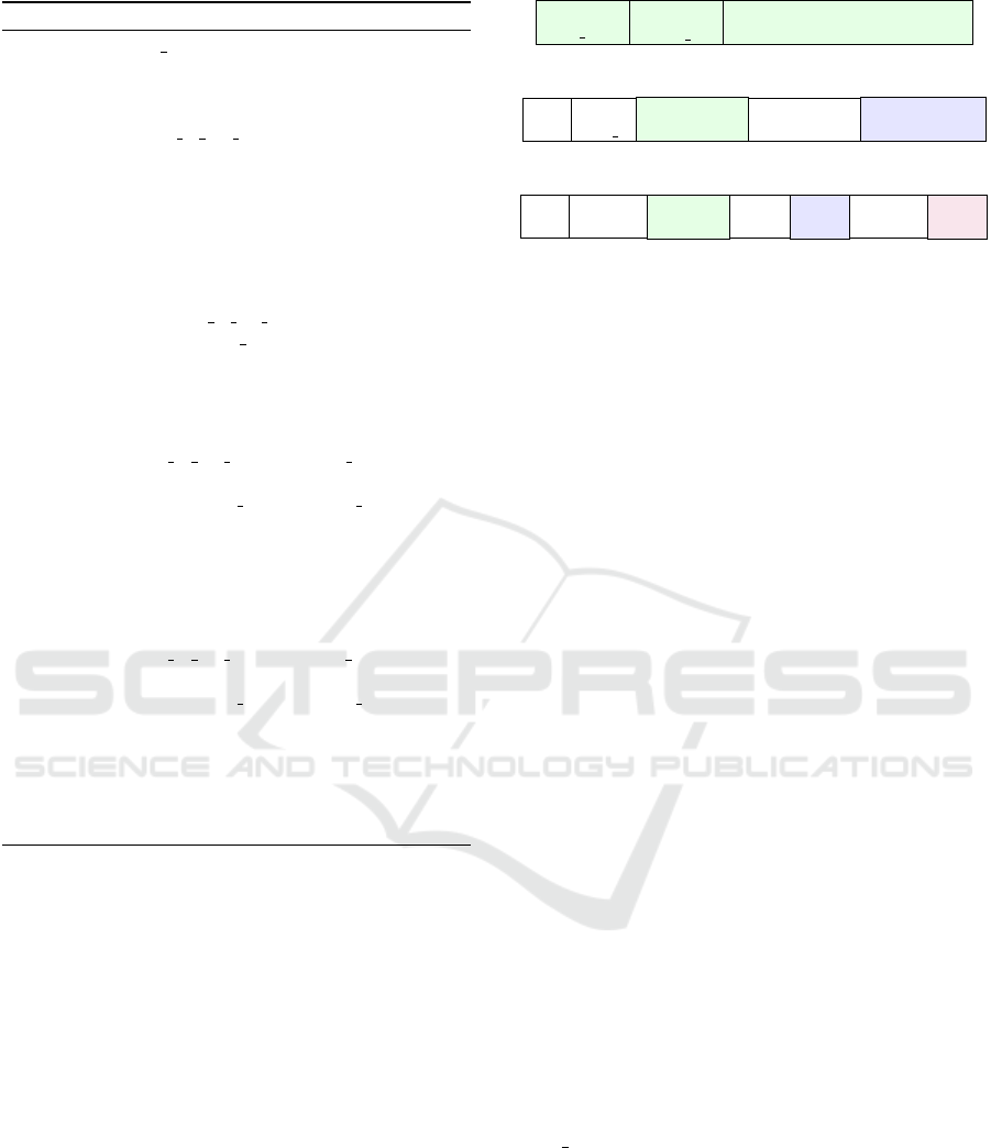
This conﬁguration at the sensor nodes forms the ex-

ternal boundary of our fog network, as computation

and storage have been pushed out into what would

traditionally be the sensor network, as shown in Fig-

ure 4. We found that the high degree of mesh density

due to clusters of sensor nodes began to compromise

the integrity of the BLE radio, in addition to being

extremely wasteful with a high volume of redundant

message transfers (a characteristic of message ﬂood-

ing). We explore this more in Section 3.2.4. As a re-

sult, we deployed a simple route selection algorithm

to maintain at most one outgoing connection per mesh

node. To support node authentication, the network is

formed from the central authentication authority out-

ward, detailed in Section 2.2.1.

VEHITS 2019 - 5th International Conference on Vehicle Technology and Intelligent Transport Systems

214

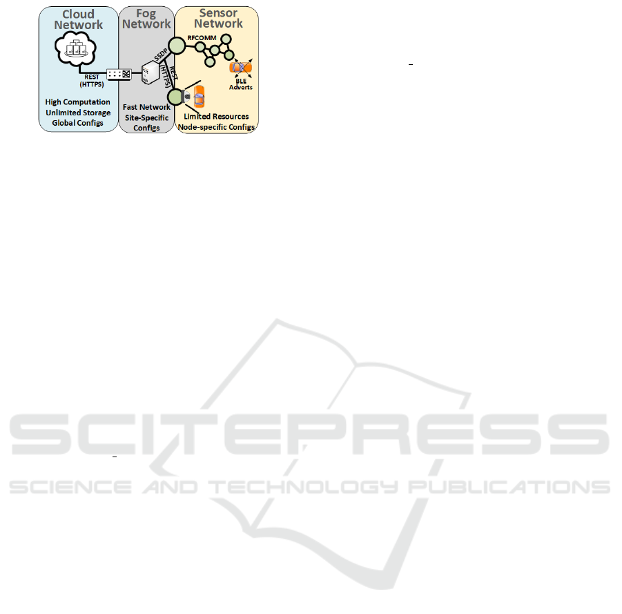
Figure 4: Fogged Network Arrangement.

2.2.1 Self-forming Authenticated Routed Mesh

Each node contains a conﬁguration (using a service

list) that speciﬁes permissions to connect to EDR

(Bluetooth) or Fog (wired Ethernet) networks. Node

discovery and network construction operate differ-

ently for these networks, as each contains different

protocols and independent physical layers. All con-

ﬁgured nodes enter a network formation phase upon

boot up and are required to authenticate with the cen-

tral node prior to being allowed to join the network

and send messages. To ensure that a path exists on

the existing network back to the central node to sup-

port authentication, the network is formed outward

from the central node, until every node in the network

has a valid link. Major functions in the network con-

struction process are shown in Algorithm 3. When a

node boots up, join network (line 1) is called, initi-

ating discovery steps for a fog network (lines 2-8) or

Bluetooth mesh network (lines 9-18). Initially, only

the central node advertises its services (both fog and

EDR Bluetooth mesh). Fog network advertisements

use a stripped down SSDP service (Seymer et al.,

2019) implemented in Python using multicast group

address 239.255.255.250, port 1900 (line 3). When

services are found, the new node and the existing net-

worked node are mutually authenticated (lines 5-6,

procedure outlined in lines 19-27) over the networked

node’s RESTful API (lines 21-27). If authentication

is successful, the new node launches its RESTful API

(line 8) written in Python and Flask (over HTTPS

on port 443) to enable bidirectional communication.

For the Bluetooth Mesh network, we use a BLE bea-

con to facilitate node discovery (line 10), rather then

our previously used (Seymer et al., 2019) SDP ser-

vice protocol, as current software support for RSSI

measurements is limited to BLE. For each node dis-

covered (line 11) that has a sufﬁciently strong signal

(line 12), authentication (line 13, procedure outlined

in lines 18-36) is performed. If authentication is suc-

cessful, node connection information is stored (line

14) so connections can be made in the future to send

messages.

We solve both the central path dependency for au-

thentication and mesh density reduction (Section 3

problems for the Bluetooth based network with the in-

troduction of a simple route generation algorithm (in

procedure join network) for the edr network. Only

nodes with an RSSI value on their advertisements

above -75dBm are considered for authentication. Af-

ter nodes are authenticated, the new node only cre-

ates an outgoing message queue for the node with the

best connection (e.g. the largest RSSI advertisement

value) (lines 15-18). Additional nodes are stored (line

14), in case this node fails so that the network is main-

tained. This forces all nodes to have at most one out-

going message queue, and only send messages to a

single networked node, reducing the overall network

density and creating forward routes for each node.

Experiments that lead us to this design are found in

Section 3. Fog connections are made over Ethernet,

and do not have such a density reduction requirement.

However we assume that the central node is in the

same broadcast domain as all other fog nodes (pre-

venting the central path dependency problem, as ev-

ery node is observable from one another during the

SSDP protocol). We see expansion of robustness for

these solutions as future work.

2.2.2 Reliable Encrypted Message Transfer

Each node pre-exchanges an AES and HMAC keys

with the central node to support message encryp-

tion (AES) and signature based integrity checking

(HMAC-SHA256), stored locally within each node.

Messages are of two main types, authentication mes-

sages and parking system messages. Authentication

messages are used to authenticate new nodes to the

mesh network, and parking system messages support

the camera, BLE space occupancy, and network

housekeeping. Each message follows the same

format (Figure 5) but differs in ﬁelds based on the

type of message being sent. This format is limited

to a single AES block size (128 bit), and begins with

a 4 bit ﬁeld indicating the message type (0000 for

heartbeats, 0001 for BLE RSSI messages, 0010 for

camera object recognition events, 0011 for message

acknowledgements, 0100 for authentication related

messages, and 0101 - 1111 reserved for future use.).

This message type helps to ensure the message is

properly parsed on the receiving end. The next ﬁeld

is a 16 bit node identiﬁer, indicating which node sent

the message. The remaining 108 bits contain the mes-

sage text being delivered. This entire 128 bit message

is encrypted and signed using the originator’s shared

AES and HMAC keys. This grows the message to

530 bits (Figure 6). When authenticating new nodes

to the network, non-central nodes will need to relay

this message to the central node, and provide it’s own

Smart Parking Zones using Dual Mode Routed Bluetooth Fogged Meshes

215

Algorithm 3: RSSI based authenticated meshnet formation.

1: procedure join network

2: if node contains ”fog” service then

3: do SSDP on Ethernet network (for 20 mins)

4: for each fog node fn found do

5: if auth to fog network(fn) then

6: initialize message queues for fn

7: if at least one fog node found then

8: launch RESTful API listener (ﬂask)

9: if node contains ”edr” service then

10: perform BLE scan (for 20 mins)

11: for each advert bn with matching UUID do

12: if bn avg RSSI ≤ -75 dBm then

13: if auth to ble network(bn) then

14: known nodes.append(bn)

15: if at least one node bn found then

16: broadcast BLE advertisements (for 20 mins)

17: gw ← bn with largest RSSI value

18: Initialize message queues for gw

19: procedure auth to fog network(node info fn)

20:  this is run by the new node

21: authmsg ← construct authentication message

22: Open RESTful HTTPS connection to fn

23: POST authmsg

24: authreply ← HTTP reply from POST

25: if authreply is valid then

26: return True

27: return False

28: procedure auth to ble network(node info bn)

29:  this is run by the new node

30: authmsg ← construct authentication message

31: Open RFCOMM connection to bn

32: Send authmsg

33: authreply ← Receive from bn

34: if authreply is valid then

35: return True

36: return False

encryption and signing to ensure secure message de-

livery. This additional pair of operations grows these

messages to 802 bits (Figure 7). To assist the cen-

tral node in choosing the appropriate keys when vali-

dating encrypted and signed message, these message

types are pre-pended with a plaintext node ID cor-

responding to the correct key identiﬁer in its key-

store (known to each node). Additionally, to assist

with routing without requiring each node to set up its

own inter-node channels, these message are also pre-

pended with a 2 bit mode identiﬁer, indicating if the

message is for the central node, or for one of the sen-

sor/relay nodes. Each of these pre-pended ﬁelds is

included in the inputs to the signature hash function.

While these ﬁelds make each message slightly larger,

the use of these shortcuts greatly improved ease of

message handling and routing implementation, and

reduces encryption/decryption related computational

demand on the low-power sensor nodes. Parking sys-

tem messages are always routed to the central node.

4 bits

msg type

16 bits

node id

108 bits

payload

Figure 5: 128 bit Message (plaintext).

2 bits

mode

16 bits

node id

128 bits

Ciphertext

128 bits

256 bits

Signature

Figure 6: 530 bit Encrypted and Signed Message.

2 bit

mode

16 bit

node id 1

128 bit

ciphertext

128 bit

256 bit

sig. 1

16 bit

node id 2

256 bit

sig. 2

Figure 7: 802 bit Relayed Node Auth Message (encrypted).

When a valid message is sent to the central node, an

encrypted and signed reply message is sent back to

the originating node, containing an identical sequence

number for the original message. If a node does not

receive an acknowledgement within a timeout period,

it resubmits the same message. This arrangement ef-

fectively doubles the message load on the network,

and we leave optimization of this to future work.

3 EXPERIMENTS

Our experimental platform consists entirely of Rasp-

berry Pi 3s, running Ubuntu Mate. Due to per-

formance problems in using Pi’s built-in Bluetooth

adapter in dual-mode, we replaced it with an after

market Bluetooth USB dongle StarTech (StarTech,

2018) to regain expected Bluetooth performance.

Our code is written in Python using the pybluez

library (karulis, 2018) and Bluez Linux Bluetooth

stack (Holtmann and Hedberg, 2018). For our local-

ization experiments, we constructed several datasets

for training and testing. Initial space ﬁngerprint-

ing used a tripod mounted beacon (at the approxi-

mate height of a vehicle’s rear view mirror) to cre-

ate vehicle model independent ﬁngerprints, but later

found that attenuation difference when the beacon

was placed in a car resulted in a poor prediction

model. We show these results in Section 3.1 and dis-

cuss our study of in-vehicle attenuation more thor-

oughly in Section 3.1.3. The complete lot was re-

ﬁngerprinted with the beacon inside a Nissan 370Z

(370 o dataset). Additional vehicles (Nissan 350Z,

Acura TL, and Nissan Rogue) were used to make

partial-lot test datasets collected locally at each node,

and over the mesh network. We refer to data collected

from nodes and transmitted over the mesh network to

the central node, as mesh datasets, and conﬁned the

size of the dataset to randomly selected spaces from

each zone. To study the effects of the mesh network

on localization, we also constructed datasets collected

directly at each node (ofﬂine, after the experiment) in

VEHITS 2019 - 5th International Conference on Vehicle Technology and Intelligent Transport Systems

216

the absence of the mesh network. We refer to these

as ofﬂine datasets. These datasets are summarized

in Table 1, with sample rates explained later in Sec-

tion 3.2.3. set1 spaces include 8, 20, 25, 27, 34, 36,

44, 53, 58, 64, 75, and 83. set2 spaces includes 25,

27, 29, 34, 36, 38, 39, 56, 58, 60, 62, 64, 67, 70, 71,

75-77, 79-81, and 87-89. set3 includes 1-2, 4, 6, 10-

13, 18, 20, 24, 31-33, 35, 37, 39-45, 49-50, 53-55,

64, 66, 68, 72, 75, 77-78, 80, 82, and 90. set4 spaces

includes 25, 27, 29, 34, 36, 56, 58, 60, 71, 72, and

75-76.

Table 1: Dataset Space Composition (of 90 total spaces).

Name Source Spaces Collect Rate

Tripod Tripod all but 84-88 Ofﬂine Constant

350 o 350Z set2 Ofﬂine Constant

370 o 370Z all (1-90) Ofﬂine Constant

TL o Acura set3 Ofﬂine Constant

350 m1 350Z set4 Mesh Constant

350 m2 350Z set1 Mesh Constant

350 m3 350Z set1 Mesh 60s sample

370 m 370Z set1 Mesh 60s sample

Rogue m Rogue set1 Mesh 60s sample

Prior experiments used the entire target parking

lot (Seymer et al., 2019). Our current experiments

removed Zone 3 (see Figure 3) due to un-relocatable

physical obstacles in those spaces. We also sought the

opportunity to deploy additional beacons compared to

past work, allowing us to study the effect of additional

RSSI datapoints on prediction accuracy, described in

the next section.

3.1 Improved Prediction Model

In prior work we found that a Random Forest algo-

rithm produced the most accurate predictions com-

pared to similar classiﬁers, and we continue to use

that algorithm in this work. However we made sev-

eral improvements to our model based on what we

learned in our experiments. We outline each of these

improvements, along with our reasoning, in this sub-

section.

3.1.1 Initial Improvements to Model and

Feature-set

We reduced our feature-set after experiments deter-

mined that only the maximum RSSI value within a

time window consistently produced accurate results.

This resulted in our feature vector shrinking from 38

in prior work, to 10 total features per time interval.

After taking RSSI measurements for each space in the

lot, we constructed a random forest model based on

these 10 features, and summarize results in Table 2.

Here we see three models trained with the tripod (tri)

dataset, and used with TL o, 350 o, and 370 o in-

vehicle datasets. Columns TP and R show True Posi-

tive percentage and ROC area, respectively. The ﬁrst

model is a Random Forest model with default settings

(no random tie breakers, iteration total of 100), with

optimized models that are conﬁgured to randomly se-

lected ties found by the algorithm, with total itera-

tions set to 1000 and 1500 (respectively). All models

use 10-fold cross-validation (CV). We use this same

model evaluation and tuning strategy throughout this

work, so that we can study the effect of model tuning

on prediction accuracy. The results of this experiment

show that while the model evaluates to 100% accu-

racy (in the second optimized case), it is only suc-

cessful at predicting other vehicles’ space occupancy

by between approximately 8% and 14%, decreasing

with our model optimization strategy. This is similar

to the results from our prior experiments, and clearly

requires improvement to make this a viable solution,

even after introducing additional sensor nodes as we

have done in this work.

Table 2: Initial Per-Space Tripod (tri) Model Results.

Model

Default Optimized 1 Optimized 2

(Dataset) TP R TP R TP R

tri 99.88% 1 99.96% 1 100.0% 1

tri(TL o) 11.23% 0.80 10.96% 0.87 10.44% 0.87

tri(350 o) 8.94% 0.79 8.94% 0.80 8.18% 0.83

tri(370 o) 14.05% 0.74 10.99% 0.81 10.91% 0.82

3.1.2 Zone based Occupancy Detection

After closely analyzing the speciﬁc error cases in our

last experiment, we surmised that we could improve

our solution accuracy if we migrated from a per-space

to a zoned based space occupancy strategy. In this

case, the parking provider cares more about the area

of the lot a vehicle is in than the individual space. In

theory, this should improve our results in cases where

the predicted space is near the true space. Using the

same data, we divided up the lot into zones as de-

ﬁned in Section 2.1.1, and re-labeled our dataset ac-

cordingly and trained a new zone-based model. Our

results are shown in Table 3. While this signiﬁcantly

improved the results, for some vehicles there was little

improvement, and overall still below acceptable accu-

racy.

3.1.3 In-vehicle Effects on Beacon Attenuation

After re-examining our testing results, we noticed that

there was an inconsistent decrease in RSSI values

when comparing the tripod’s signature with the in-

vehicle signature. When the beacon is located on a

Smart Parking Zones using Dual Mode Routed Bluetooth Fogged Meshes

217

Table 3: Initial Zone Based Tripod (tri) Model Results.

Model

Default Optimized 1 Optimized 2

(Dataset) TP R TP R TP R

tri 99.68% 1 99.68% 1 99.68% 1

tri(TL o) 42.46% 0.83 38.77% 0.83 38.95% 0.82

tri(350 o) 16.06% 0.71 18.33% 0.77 18.48% 0.77

tri(370 o) 43.33% 0.81 43.93% 0.82 43.93% 0.82

tripod, it physically approximates the location of the

beacon if it were mounted in a vehicle, however the

effect of the vehicle’s surrounding structure appeared

to differ depending on the direction of the vehicle’s

orientation with respect to our sensor nodes. For ex-

ample, in every case we examined, the nodes facing

the rear of the vehicle had the most signiﬁcant effect

on RSSI value, followed by nodes that faced to the

left or right of the vehicle. Nodes in front of the ve-

hicle had the least attenuation effect, approximately

1 RSSI in most cases. We quickly realized that the

materials in the vehicle produced this effect, due to

the orientation of our beacon (placed behind the vehi-

cle’s rear-view mirror). To the front and sides of the

vehicle, transmission was most often through a single

pane of autoglass. To the rear of the vehicle, it was

often through seats, metal, and in most cases the rear-

view mirror itself, resulting in as much as a 6 RSSI

decrease. In prior work, we globally increased all

recorded RSSI values to compensate for some of this

attenuation, however, improvements were limited and

inconsistent. Our current experiments and analysis

add clarity to this result. We used a tripod for ﬁnger-

printing so that we didn’t introduce a vehicle-speciﬁc

bias into our model, however the consequence of in-

consistent in-vehicle beacon attenuation became our

limiting factor. Our solution was to replace the tripod

dataset with a model constructed from beacon mea-

surements inside a vehicle. We selected the 370Z, due

to convenience and availability of the vehicle, but ac-

knowledge that the physical placement of the beacon

may produce positive results only for similarly ori-

ented vehicles (i.e. larger vehicles may need to have

their own radio map). We discuss experiments with

the in-vehicle model in the next subsection.

3.1.4 In-vehicle Fingerprinting

After re-ﬁngerprinting the lot with the 370Z, we

trained new models, and repeated our per-space tests

as they provide better insight into the cause of fail-

ures. Results are shown in Table 4. Here we see

a similarly valid trained model with accuracy above

99% in all cases. Testing results for the Acura and

350Z also improved, in some cases signiﬁcantly, al-

though the need for zone-based detection was clearly

still needed.

Table 4: Per-Space In-Vehicle (370) Fingerprinting Results.

Model

Default Optimized 1 Optimized 2

(Dataset) TP R TP R TP R

370 99.63% 1 99.56% 1 99.56% 1

370(TL o) 42.11% 0.92 40.79% 0.95 40.79% 0.95

370(350 o) 12.78% 0.85 13.75% 0.89 13.19% 0.89

We also recomputed these results using the zoned

scheme described in Section 3.1.2, and show results

in Table 5. Here we see marked improvements over-

all, with the default model achieving the highest accu-

racy. All tests produced results with ROC area above

0.99. This degree of accuracy, while not perfect in

all cases, is high enough that we proceeded with con-

structing the remainder of the solution around them.

We proceeded with mesh experiments in the next sub-

section.

Table 5: Zoned In-Vehicle (370) Fingerprinting Results.

Model

Default Optimized 1 Optimized 2

(Dataset) TP R TP R TP R

370 99.78% 1 99.67% 1 99.67% 1

370(TL o) 89.65% 0.99 89.39% 0.99 89.39% 0.99

370(350 o) 85.28% 1.0 79.86% 1 79.86% 1

3.2 Over-mesh Experiments

Our initial mesh experiments used a managed ﬂood-

ing algorithm without our routing feature, and used

parameters that were extremely permissive in both

node link creation and message volume which re-

sulted in some areas of our mesh becoming very

dense. This section outlines experiments of our self-

forming mesh network, and our improvements that

lead to the sampled routing outlined in Section 2.

3.2.1 Self Forming Experiment

Recall our node deployment in Figure 3. When we

activated our mesh network nodes and the network

formed with our initial set of parameters, we noticed

that the mesh was not well formed. The network be-

came extremely dense and highly dependent on node

1. Additionally, no EDR nodes were observable by

node 8, resulting in the fog network and EDR net-

work being very isolated, routing exclusively through

node 1. Our solution was to deploy an EDR-only (no

vehicle sensing conﬁguration) node (called node 10)

to a midpoint between node 8 and it’s nearest (but not

BLE observable) neighbor, node 4. This allowed us to

provide a redundant network path, lessening the risk

from the single path through node 1. We were also

able to more easily manipulate connection thresholds

due to this additional path, and discuss this further in

Sections 3.2.2 and 3.2.3.

VEHITS 2019 - 5th International Conference on Vehicle Technology and Intelligent Transport Systems

218

3.2.2 Prediction Over-mesh Experiments

Once our mesh network was established, we per-

formed beacon collection with the 370Z as our test

vehicles (to temporarily remove error due to vehicle

differences), and ran prediction tests using our cur-

rent model while collecting data from the central node

(since the network now existed to route data back to

it). Our preliminary results are shown in Table 6. We

examined the data used in this result, as well as mes-

sage collection metrics and other instrumentation, and

noticed large effects on the observability of beacons

in our mesh conﬁguration. As both the EDR network

and the beacon scanning shared the same radio, one

could not function while the other was in use, result-

ing in fewer beacons being observed due to the load

placed on the radio by the mesh network. There was

also a very long delay in transmission of all beacons,

an effect that increased over time due to the inefﬁ-

ciently managed ﬂooding algorithm we were using.

We also show the zoned version of our result in Ta-

ble 6. While improvements were seen, this result was

worse than data collected locally. After examining

the data, we noticed that most of the data collected

had gaps in observations from some nodes, causing

the model to perform poorly.

We concluded from these results that we must

ﬁnd a way to reduce the number of messages routed

through the network. This would result in less mes-

sage ﬂooding, providing more on-radio time for the

beacon receiver. We reprocessed our data to take the

maximum RSSI value for the entire observation win-

dow (of 5 minutes), and use that as a single predic-

tion case, instead of the 10-second time intervals we

had been using, as such windows were too short for

the beacon to be seen by any given node. We show

this in the same table, as Single Max. This resulted

in some improvement, but still below our non-mesh

result. This suggested, however, that sampling our

beacons to reduce message volume, may result in a

viable solution that would improve performance.

Table 6: Initial Over-Mesh Predication Results.

Model (Dataset) TP R

370 Per-Space (350 m1) 1.98% 0.60

370 Per-Space (350 m2) 9.72% 0.82

370 Per-Space (350 m1 Single Max) 8.33% 0.85

370 Per-Space (350 m2 Single Max) 8.33% 0.91

370 Zoned (350 m1) 46.33% 0.82

370 Zoned (350 m2) 61.94% 0.85

370 Zoned (350 m1 Single Max) 66.67% 0.68

370 Zoned (350 m2 Single Max) 75% 0.75

3.2.3 Message Down-sampling Experiments,

effects on prediction

To gain insight into the effects of down-sampling

without re-implementing our code, we took our in-

vehicle ﬁngerprinting set and compiled several train-

ing sets, each with different sample rates. We chose to

favor heavily sampled sets, and chose 30, 60, 120, and

300 seconds as our sample rates. Results are shown

in Table 7. Here we see that all of our sampling rates

produced a highly accurate model, however we saw

diminishing returns when we passed the 60 second

sampling rate. We then re-implemented our mesh net-

work and beacon sampling solution with this rate, and

repeated our experiments with additional test vehi-

cles. The results are described in the next subsection.

Table 7: 370 Down-sampled Per-Space Results.

Model(dataset) TP R Model(dataset) TP R

370 (370 30s) 99.78% 1 370 (370 60s) 99.78% 1

370 (370 120s) 98.33% 1 370 (370 300s) 97.78% 1

3.2.4 Sampled and Routed Mesh Results

Prior to implementing our sampling solution in our

mesh network code, we attempted to resolve the radio

use problem by introducing sender invocation delays

in our mesh network, so that messages could queue

up on a node, then burst across to other nodes when

the sender established a connection. We performed an

experiment with this parameter in place with the 350

(constructing the 350 m3 dataset). We show this re-

sults in the ﬁrst row of Table 8. This resulted in fewer

invocations of EDR connections, further reducing de-

mand on the radio. We also noticed that the mesh

network was introducing a large delay in the time the

central node received all of the messages needed to

make a prediction decision. While these were accept-

able, they were still not ideal, as these delays will

need to be increased as load increases. Such an ar-

rangement will not scale with more beaconing vehi-

cles entering the lot.

Instead we introduced a node selection and rout-

ing algorithm, Algorithm 3 in Section 2.2.1, imple-

mented the sampled message scheme previously de-

termined, and repeated mesh experiments with the

370, and Nissan Rogue (to add diversity with a larger

vehicle than the smaller ones we had been using).

We used the data from the 350 o and assembled a

sampled dataset with it’s values, without repeating

the over-mesh experiment with that vehicle. With

these three mesh datasets we tested the previously

constructed 370 Zoned model shown in the ﬁrst three

lines of Table 8.

Smart Parking Zones using Dual Mode Routed Bluetooth Fogged Meshes

219

We noticed that during our analysis that there was

a slight loss in accuracy when we trained a model

based on zoned labels, when compared to a per-space

model that was relabeled after prediction. Our ﬁnal

modiﬁcation to our prediction scheme was to use the

per-space model for prediction, but match each space

with its correct zone label after prediction. We then

took the majority result as the zone our system indi-

cates the vehicle to be located in. These results are

shown in the bottom 6 lines of Table 8. Here we see

that the 350z was predicted in the correct zone for all

of our test data, while the 370 and Rogue were correct

83.33% and 75% of the time, respectively. After ex-

amining our results more closely, we determined that

the lack of perfect prediction in the 370 and Rogue

cases were the result of 3 problematic spaces in our

test set, in some cases resulting in a 50% (but not a

majority) prediction. We seek to tune our model in

the future to solve the problem with those particular

spaces.

Table 8: 60s Sampled Mesh Results (Zoned only).

Model

Default

(Dataset) TP R

370 Zoned(350 m3) 83.33% 0.90

370 Zoned(370 m) 77.08% 0.88

370 Zoned(Rogue m) 77.08% 0.90

370 60s Post Zoned (350 m3) 95.83% -

370 60s Post Zoned (370 m) 85.41% -

370 60s Post Zoned (Rogue m) 75% -

370 60s Post Zoned Majority (350 m3) 100% -

370 60s Post Zoned Majority (370 m) 83.33% -

370 60s Post Zoned Majority (Rogue m) 75% -

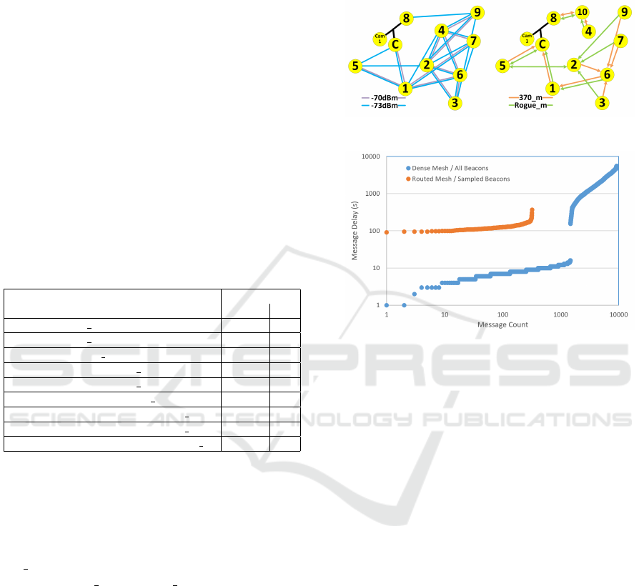
We also examined the message delay, to further val-

idate our choice to migrate from our previous man-

aged ﬂooding solution to the lower-demand routing

one. Figure 8 shows the links established in two of

our dense mesh implementations used to create the

350 m3 dataset (left) with the routed implementation

used for the 370 m and Rogue m datasets (right). The

ﬁgure show that the network itself is much less dense

with the routed solution. During our experiments, we

also recorded the timestamp for when a message was

created, and a timestamp for when the central node re-

ceived that message. We then measured the difference

between these timestamps for both the dense mesh

and routed mesh implementations, shown in Figure 9

sorted by message delay. The routed mesh shown in-

cluded the 60 second beacon sampling, causing the

lower bound of all messages to be 60 seconds. While

the dense mesh produced message delivery for some

messages much faster than the sampled and routed so-

lution (during times of low load), its upper bound was

unacceptably large (more than an hour in some cases).

Consequently we selected the routed, sampled, imple-

mentation as our end solution, due to our results and

the expectation that as this solution scales well to mul-

tiple vehicles on a lot.

Figure 8: Dense Mesh vs. Routed Mesh.

Figure 9: Message Delay Comparison.

3.3 Camera vs. BLE based Vehicle

Entrance/Exit Detection

Our last set of experiments compares the use of the

object recognition camera based vehicle entrance and

exit detection (outlined in Section 2.2.1) with a BLE

only solution. We conducted a series of 10 instances

where the 370Z was driven into and out of the lot at a

constant speed of 10 mph, making one traversal in the

camera’s ﬁeld of view, and its BLE beacon receiver

range. We found that -70 dBm was a consistent value

to use as a threshold for determining when the vehi-

cle passed by this node. We summarize the number

of beacons observed, the number of times the object

recognition camera recognized the vehicle as a car,

and the range of delay between when the beacon was

seen, and when the camera produced a detection event

over its serial connection in Table 9. This delay was

computed by attempting to match a beacon event with

a camera event, and measuring the time difference.

There is a consistent delay of several seconds from

when the vehicle passes in front of the camera, and a

detection decision is made. We also see that both the

camera and BLE beacon receiver observe a single ve-

hicle multiple times. However we also acknowledge

that if a vehicle travels too quickly it may not be de-

tected by the camera, so duplicates are welcomed.

VEHITS 2019 - 5th International Conference on Vehicle Technology and Intelligent Transport Systems

220

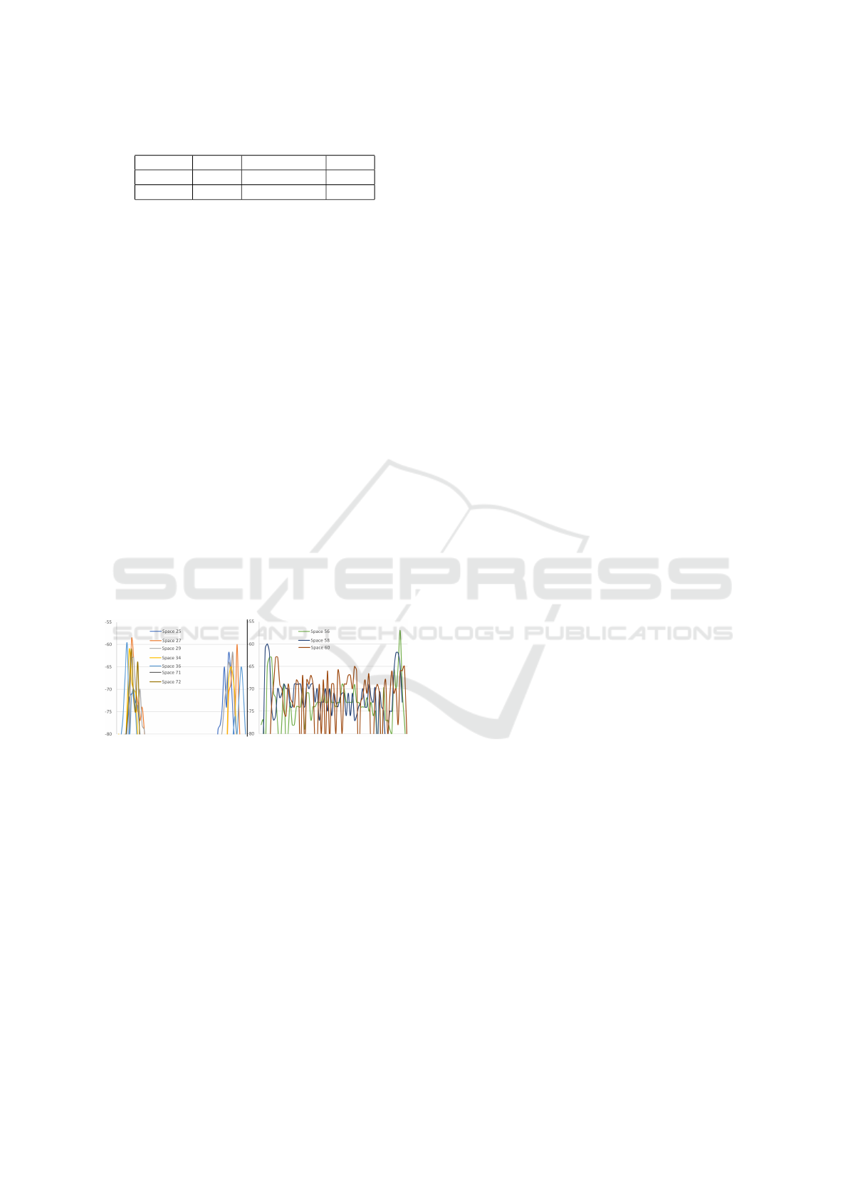
Table 9: Daytime Camera Recognition vs BLE (≤ 70 dBm).

Direction Beacons Recog. Objects delta t

Enter (10) 2-3 1-2 ”car” 0-3 sec

Exit (10) 1-4 1-3 ”car” 2-11 sec

We repeated this enter/exit experiment at night (with

no light), and found that the camera produced no de-

tection results, rendering it not usable in these con-

ditions. We coupled this experiment with other mesh

related parking experiments, including parking spaces

very near to the camera node’s beacon receiver. We

show these results in Figure 10. On the left, we see

now the camera node observes beacons for spaces far

from it, while on the right we see observations for

spaces that are close to the node. Although entrance

and exit are consistently detectable by this node, there

are false positives produced by beacon observations

of the vehicle while it’s parked, simply because those

spaces are physically close to the node. We conclude

from these experiments that the BLE solution is the

only solution that will function 24 hours a day, and

that this node was located too close to existing park-

ing spaces to make it a good discriminator for vehicle

entrance. For our chosen parking lot, the optimal so-

lution for vehicle detection would use an aggregate

from results from all nodes, rather than this particular

ingress point, reducing the impact of false positives at

any one node.

Figure 10: Night Entrance / Exit Detection.

4 RELATED WORK

Prior work with RSSI-based radio localization us-

ing IEEE 802.15.4 radio (Oguejioforo. et al., 2013)

and RSSI values used trilateration involving linear

distance calculations. Other work uses radio ﬁnger-

printing instead of distance estimation (Olevall and

Fuchs, 2017). Silver (Silver, 2016) combines vari-

ous value ﬁltering techniques and compares disc tri-

lateration and k-nearest neighbor ﬁngerprinting tech-

niques. (Daniay and Cemgil, 2017) focuses on RSSI

ﬁngerprinting of moving beacons using a combina-

tion of Wasserstein distance interpolation, k-nearest

neighbor, and Neural Networks. Radio selection is

diverse as well, with Faragher and Harle comparing

use of BLE and WiFi (Faragher and Harle, 2014).

Additional indoor wireless positioning techniques are

found in (Liu et al., 2007). Initially, we used a con-

trolled ﬂooding algorithm similar to the Bluetooth

SIG BLE mesh speciﬁcation (ble, 2017), however

our solution uses Bluetooth classic (EDR) instead of

BLE to transmit network messages. Additional ﬂood-

ing (Kim et al., 2015) and routed Bluetooth mesh net-

works are surveyed in (Darroudi and Gomez, 2017)

Research in Smart Parking systems encompasses

many aspects of parking management including space

occupancy detection, space availability prediction,

payment management, rule violation alerts, and much

of the IT infrastructure used to connected these as-

pects into a uniﬁed system. (Liniger, 2015) uses

GPS-based localization augmented by mobile phones

and BLE beacons. This information is combined with

the vehicle’s On-Board Diagnostic (OBD-2) data to

measure the state of the vehicle (speed, etc.). (Fabian,

2015) provides a solution that uses BLE trilatera-

tion to develop a local parking management solu-

tion. Yee et al. (Yee and Rahayu, 2014) uses Zig-

bee radios. Some solutions on dead reckoning and

other navigation-based solutions, such as those found

within smartphone inertial sensors (Gao et al., 2017)

that beneﬁt from no requirement to modify the inter-

nal space, but controlled by the vehicle owner, making

localization results untrustworthy. Other solutions use

historic data or and crowd-sourced GPS information

to estimate space occupancy (Hobi, 2015).

Several parking management solutions that use

per-space sensing based on Radio-frequency iden-

tiﬁcation (RFID), optical, or magnetic technologies

have been suggested (Mainetti et al., 2015; Gandhi

and Rao, 2016; Patil and Bhonge, 2013; Sadhukhan,

2017) but lack experimental validation or details on

communication and other protocols used. The viabil-

ity of these solutions are hard to compare with ours,

due to the apparent lack of experimental rigor. In-

stead we use Random Forest classiﬁers for radio lo-

calization. Additional examples of the diversity in ap-

plications of Random Forest classiﬁers (beyond park-

ing prediction) can be found in (Belgiu and Dragut,

2016).

5 CONCLUSION

We provide a reliable and accurate system to de-

termine zone-based parked vehicle occupancy and

convey that information to external networks using

only Bluetooth radio. Our zone-based solution is

shown to be more accurate than per-space determi-

Smart Parking Zones using Dual Mode Routed Bluetooth Fogged Meshes

221

nations. We designed a means to integrate camera-

based object recognition into our system to provide

additional vehicle attestation options, and performed

an experiment-based comparison of this implementa-

tion to our BLE-only solution. Outdoor parking lot

owners can use solutions like ours to cheaply and eas-

ily deploy seamless smart parking solutions.

ACKNOWLEDGEMENTS

The author’s afﬁliation (pseymer@mitre.org) with

The MITRE Corporation is provided for identiﬁca-

tion purposes only, and is not intended to convey or

imply MITRE’s concurrence with, or support for, the

positions, opinions, or viewpoints expressed by the

author. Approved for Public Release 19-0071. Distri-

bution Unlimited.

REFERENCES

(2017). Bluetooth mesh proﬁle speciﬁcation.

Belgiu, M. and Dragut, L. (2016). Random forest in remote

sensing: A review of applications and future direc-

tions. ISPRS Journal of Photogrammetry and Remote

Sensing, 114:24 – 31.

Daniay, F. S. and Cemgil, A. T. (2017). Model-based local-

ization and tracking using bluetooth low-energy bea-

cons. Sensors, 17(11).

Darroudi, S. M. and Gomez, C. (2017). Bluetooth low en-

ergy mesh networks: A survey. Sensors, 17(7):1467.

Fabian, H. (2015). A public parking management system

for zurich. Master’s thesis, University of Zurich.

Faragher, R. and Harle, R. (2014). An analysis of the ac-

curacy of bluetooth low energy for indoor positioning

applications. In Proceedings of the 27th International

Technical Meeting of The Satellite Division of the In-

stitute of Navigation (ION GNSS+ 2014), pages 201 –

210, Tampa, Florida.

Gandhi, B. M. K. and Rao, M. K. (2016). A prototype for

iot based car parking management system for smart

cities. Indian Journal of Science and Technology,

9(17).

Gao, R., Zhao, M., Ye, T., Ye, F., Wang, Y., and Luo, G.

(2017). Smartphone-based real time vehicle tracking

in indoor parking structures. IEEE Transactions on

Mobile Computing, 16(7):2023–2036.

Hobi, L. (2015). The impact of real-time information

sources on crowd-sourced parking availability predic-

tion. Master’s thesis, University of Zurich.

Holtmann, M. and Hedberg, J. (2018). Bluez - ofﬁcial linux

bluetooth protocol stack.

Itti, L. (2018). Darknet yolo jevois module.

JeVois Inc (2018). Jevois-a33 smart camera.

karulis (2018). Pybluez - python extension module allowing

access to system bluetooth resources.

Kim, H., Lee, J., and Jang, J. W. (2015). Blemesh: A wire-

less mesh network protocol for bluetooth low energy

devices. In 2015 3rd International Conference on Fu-

ture Internet of Things and Cloud, pages 558–563.

Liniger, S. (2015). Parking prediction techniques in an iot

environment. Master’s thesis, University of Zurich.

Liu, H., Darabi, H., Banerjee, P., and Liu, J. (2007). Sur-

vey of wireless indoor positioning techniques and

systems. IEEE Transactions on Systems, Man,

and Cybernetics, Part C (Applications and Reviews),

37(6):1067–1080.

Mainetti, L., Patrono, L., Stefanizzi, M. L., and Vergallo,

R. (2015). A smart parking system based on iot pro-

tocols and emerging enabling technologies. In 2015

IEEE 2nd World Forum on Internet of Things (WF-

IoT), pages 764–769.

Oguejioforo., S., Okorogu, V., Abe, A., and OsuesuB., O.

(2013). Outdoor localization system using rssi mea-

surement of wireless sensor network. In International

Journal of Innovative Technology and Exploring En-

gineering, volume 2.

Olevall, A. H. and Fuchs, M. (2017). Indoor navigation and

personal tracking system using bluetooth low energy

beacons. Master’s thesis.

Patil, M. and Bhonge, V. N. (2013). Wireless sensor net-

work and rﬁd for smart parking system.

Redmon, J. and Farhadi, A. (2018). Yolov3: An incremental

improvement. arXiv.

Sadhukhan, P. (2017). An iot-based e-parking system for

smart cities. 2017 International Conference on Ad-

vances in Computing, Communications and Informat-

ics (ICACCI), pages 1062–1066.

Seymer, P., Wijesekera, D., and Kan, C.-D. (2019). Se-

cure outdoor smart parking using dual mode bluetooth

mesh networks. In 89th IEEE Vehicular Technology

Conference.

Silver, O. (2016). An indoor localization system based on

ble mesh network. Master’s thesis, Link

oping Univer-

sity.

StarTech (2018). Mini usb bluetooth 4.0 adapter - 50m

(165ft) class 1 edr wireless dongle.

Yee, H. C. and Rahayu, Y. (2014). Monitoring parking

space availability via zigbee technology. Interna-

tional Journal of Future Computer and Communica-

tion, 3(6):377.

VEHITS 2019 - 5th International Conference on Vehicle Technology and Intelligent Transport Systems

222

REFERENCES

(2017). Bluetooth mesh profile specification.